 |
The SKIRT project
advanced radiative transfer for astrophysics
|
|
The SKIRT project
advanced radiative transfer for astrophysics
|
This tutorial introduces the time lag tracking capabilities of the SKIRT code (see Tracking time lags with SKIRT). You will examine X-ray reverberation mapping, a technique used to estimate the time lag between direct and reprocessed emission in an active galactic nucleus (AGN). In this model, the AGN is represented by cold gas in a parsec-scale torus surrounding a central source. You will create a ski file containing the appropriate simulation parameters, perform the SKIRT simulation, and analyze the results, focusing on the time lag and X-ray spectra in the 2 to 12 keV range.
This tutorial assumes that you have completed the introductory SKIRT tutorial X-ray reprocessing in a clumpy AGN torus and that you have reviewed the topic Tracking time lags with SKIRT, or that you have otherwise acquired the working knowledge introduced there. At the very least, before starting this tutorial, you should have installed the SKIRT code.
In a terminal window, with your local working directory as the current directory, start SKIRT without any command line arguments. SKIRT responds with a welcome message and starts an interactive session in the terminal window, during which it will prompt you for all the information describing the simulation:
   Welcome to SKIRT v___
   Running on ___ for ___
   Interactively constructing a simulation...
 ? Enter the name of the ski file to be created: reverberation
The first question is for the filename of the ski file. For this tutorial, enter "reverberation".
   Possible choices for the user experience level:
      1. Basic: for beginning users (hides many options)
      2. Regular: for regular users (hides esoteric options)
      3. Expert: for expert users (hides no options)
 ? Enter one of these numbers [1,3] (2): 2
As discussed in a previous tutorial (see Experience level), the Q&A session can be tailored to the experience level of the user. For this tutorial, select the Regular level.
   Possible choices for the units system:
      1. SI units
      2. Stellar units (length in AU, distance in pc)
      3. Extragalactic units (length in pc, distance in Mpc)
 ? Enter one of these numbers [1,3] (3): 3
   Possible choices for the output style for wavelengths:
      1. As photon wavelength: λ
      2. As photon frequency: ν
      3. As photon energy: E
 ? Enter one of these numbers [1,3] (1): 3
   Possible choices for the output style for flux density and surface brightness:
      1. Neutral: λ F_λ = ν F_ν
      2. Per unit of wavelength: F_λ
      3. Per unit of frequency: F_ν
      4. Counts per unit of energy: F_E
  ? Enter one of these numbers [1,4] (4): 4
As discussed in a previous tutorial (see Units), SKIRT offers several options for the output units. In this tutorial, you will be modelling an AGN, so select extragalactic units (the default option). In the X-ray range, you want to use photon energies in keV as the spectral variable, and photon counts per energy as the flux output style.
   Possible choices for the overall simulation mode:
      1. No medium - oligochromatic regime (a few discrete wavelengths)
      2. Extinction only - oligochromatic regime (a few discrete wavelengths)
      3. No medium (primary sources only)
      4. Extinction only (no secondary emission)
      5. Extinction only with Lyman-alpha line transfer
      6. With secondary emission from dust
      7. With secondary emission from gas
      8. With secondary emission from dust and gas
 ? Enter one of these numbers [1,8] (4): 4
As discussed in a previous tutorial (see Simulation mode), the answer to this question determines the wavelength regime of the simulation (oligochromatic or panchromatic) and sets the overall scheme for handling media in the simulation.
The SKIRT timing capability requires one of the "Extinction only" modes, i.e. "2", "4", or "5" in the above list. Furthermore, as X-ray interactions modify the photon energy, oligochromatic simulations are not very useful in the X-ray range. For this tutorial, select "Extinction only (no secondary emission)".
? Enter the default number of photon packets launched per simulation segment [0,1e19] (1e6): 1e7
For an acceptable level of Monte Carlo noise in this tutorial, set the number of photon packets to \(10^7\) rather than the default value of \(10^6\). Further increasing this number will improve the signal to noise ratio.
   Possible choices for the cosmology parameters:
      1. The model is at redshift zero in the Local Universe
      2. The model is at a given redshift in a flat universe
 ? Enter one of these numbers [1,2] (1):
We assume a redshift of zero for the local universe.
 ? Enter the shortest wavelength of photon packets launched from primary sources ...: 50 keV
 ? Enter the longest wavelength of photon packets launched from primary sources ...: 1.9 keV
The source system requests the limits of the wavelength range to be considered for the primary sources. Keep in mind that the shortest wavelength corresponds to the highest photon energy, and vice versa. In this tutorial, you are interested in the 2 to 12 keV range. However, fluorescence in this energy range can be triggered by absorption at much higher energies, so you have to consider radiative transfer at photon energies up to 50 keV. At the lower energy limit, enter 1.9 keV to avoid any discontinuities at 2 keV.
   Possible choices for item #1 in the primary sources list:
      1. A primary point source
      2. A primary source with a built-in geometry
         ...
 ? Enter one of these numbers or zero to terminate the list [0,12] (2): 1
 ? Enter the position of the point source, x component ]-∞ pc,∞ pc[ (0 pc):
 ? Enter the position of the point source, y component ]-∞ pc,∞ pc[ (0 pc):
 ? Enter the position of the point source, z component ]-∞ pc,∞ pc[ (0 pc):
The source of primary X-ray photons (i.e. the X-ray corona of the AGN) can be modelled as a point source at the origin (the default position coordinate values).
   Possible choices for the angular luminosity distribution of the emission:
      1. An isotropic emission profile
      2. A laser emission profile
      3. An anisotropic conical emission profile
      4. A Netzer AGN accretion disk emission profile
 ? Enter one of these numbers or zero to select none [0,4] (1):
   Possible choices for the polarization profile of the emission:
      1. An unpolarized emission profile
      2. An axysimmetric sine-square polarization emission profile
 ? Enter one of these numbers or zero to select none [0,2] (1):
 ? Enter the bulk velocity of the source, x component [-1e5 km/s,1e5 km/s] (0 km/s):
 ? Enter the bulk velocity of the source, y component [-1e5 km/s,1e5 km/s] (0 km/s):
 ? Enter the bulk velocity of the source, z component [-1e5 km/s,1e5 km/s] (0 km/s):
For this tutorial, the primary radiation is assumed to be isotropic, unpolarized, and lacking bulk motion. Note that the SKIRT timing capability remains enabled even if these assumptions are not met.
   Possible choices for the spectral energy distribution for the source:
      1. A black-body spectral energy distribution
         ...
     12. A spectral energy distribution loaded from a text file
     13. A spectral energy distribution specified inside the configuration file
         ...
 ? Enter one of these numbers [1,16] (1): 13
 ? Enter the wavelengths at which to specify the specific luminosity [... keV]: 50 keV, 1.9 keV
   Possible choices for the luminosity unit style:
      1. Neutral: λ L_λ = ν L_ν
      2. Per unit of wavelength: L_λ
      3. Per unit of frequency: L_ν
      4. Counts per unit of energy: L_E
 ? Enter one of these numbers [1,4] (2): 4
 ? Enter the specific luminosities at each of the given wavelengths ]... 1/s/keV[: 2.8e-3, 1
In an actual research setting, you would probably consider an exponentially cut-off power-law spectrum for the X-ray corona. However, in this tutorial, configure the spectrum to be a straightforward power law with a negative photon index of 1.8 and arbitrary scaling (the normalization is specified in the following step). Because SKIRT log-log interpolates between wavelength points in a tabulated grid, a power-law can be specified with just two points, one at each end of the wavelength range.
Thus, you can simply use the ListSED class to specify the two outer points of the spectral range. Assuming a scale-free specific luminosity of 1 at 1.9 keV, the corresponding value at 50 keV is \((50/1.9)^{-1.8}\approx 2.8 \times 10^{-3}\). Make sure to select the option "Counts per unit of energy" to specify the power law in energy space.
   Possible choices for the type of luminosity normalization for the source:
      1. Source normalization through the integrated luminosity for a given wavelength range
      2. Source normalization through the specific luminosity at a given wavelength
      3. Source normalization through the specific luminosity for a given wavelength band
 ? Enter one of these numbers [1,3] (1): 1
   Possible choices for the wavelength range for which to provide the integrated luminosity:
      1. The wavelength range of the primary sources
      2. All wavelengths (i.e. over the full SED)
      3. A custom wavelength range specified here
 ? Enter one of these numbers [1,3] (1): 3
 ? Enter the shortest wavelength of the integration range ...: 12 keV
 ? Enter the longest wavelength of the integration range ...: 2 keV
 ? Enter the integrated luminosity for the given wavelength range ]0 erg/s,∞ erg/s[: 5e41 erg/s
Select the option to normalise the source spectrum through the integrated luminosity for a given wavelength range, choose a custom wavelength range, and specify the shortest (12 keV) and longest (2 keV) wavelengths. Finally, provide an AGN luminosity of \(5\times 10^{41}~\mathrm{erg}\,\mathrm{s}^{-1}\).
   Possible choices for item #2 in the primary sources list:
      1. A primary point source
         ...
 ? Enter one of these numbers or zero to terminate the list [0,12] (2): 0
When asked for a second source component, enter zero to terminate the list. The SKIRT timing capability remains enabled even if a second source component is added.
   Possible choices for item #1 in the transfer media list:
      1. A transfer medium with a built-in geometry
      2. A transfer medium imported from smoothed particle data
         ...
 ? Enter one of these numbers [1,7] (1): 1
   Possible choices for the geometry of the spatial density distribution for the medium:
      1. A Plummer geometry
         ...
     11. A torus geometry
         ...
 ? Enter one of these numbers [1,41] (1): 11
 ? Enter the radial powerlaw exponent p of the torus [0,∞[: 2
 ? Enter the polar index q of the torus [0,∞[: 0
 ? Enter the half opening angle of the torus [0 deg,90 deg]: 5
 ? Enter the minimum radius of the torus ]0 pc,∞ pc[: 2.4e-2 pc
 ? Enter the maximum radius of the torus ]0 pc,∞ pc[: 4.8e-2 pc
 ? Do you want to reshape the inner radius according to the Netzer luminosity profile? [yes/no] (no):
You now introduce the torus of cold gas to the simulation. Select a transfer medium with a built-in geometry (the default option). Then, select a plain (wedge) torus base geometry and configure its properties: a density profile with radial index of 2 and polar index of 0, an opening angle of 5 degrees (measured from the equatorial plane), and radii extending from \(2.4\times 10^{-2}\) to \(4.8\times 10^{-2}\) pc.
   Possible choices for the material type and properties throughout the medium:
      1. A typical interstellar dust mix (mean properties)
         ...
     19. A gas mix supporting photo-absorption and fluorescence for X-ray wavelengths
         ...
 ? Enter one of these numbers [1,20] (1): 19
 ? Enter the abundancies for the elements with atomic number Z = 1,...,30 [0,1] ():
 ? Enter the temperature of the gas or zero to disable thermal dispersion [0 K,1e9 K] (1e4 K): 0 K
Next, you select the gas mix that implements photo-absorption and fluorescence for X-ray wavelengths (see Medium system). Choose the default element abundancies by entering an empty string, and specify a temperature of zero to disable thermal dispersion.
   Possible choices for the type of normalization for the amount of material:
      1. Normalization by defining the total mass
      2. Normalization by defining the total number of entities
      3. Normalization by defining the optical depth along a coordinate axis
      4. Normalization by defining the mass column density along a coordinate axis
      5. Normalization by defining the number column density along a coordinate axis
 ? Enter one of these numbers [1,5] (3): 5
   Possible choices for the axis along which to specify the normalization:
      1. The X axis of the model coordinate sytem
      2. The Y axis of the model coordinate sytem
      3. The Z axis of the model coordinate sytem
 ? Enter one of these numbers [1,3] (3): 1
 ? Enter the number column density along this axis ]0 1/cm2,∞ 1/cm2[: 1e25
The total amount of obscuring gas in a torus is commonly expressed through the equatorial number column density of neutral hydrogen \(N_\mathrm{H}\). You can follow this convention by selecting "normalization through the number column density" and "along the X-axis". However, SKIRT normalizes the medium along the entire X-axis, while the observed value characterizes the amount of material as measured from the source outwards. Therefore, to model a torus with \(N_\mathrm{H} = 5 \times 10^{24}~\mathrm{cm}^{-2}\), you must specify twice this value in SKIRT.
   Possible choices for the spatial distribution of the velocity, if any:
      1. A vector field pointing away from the origin
      ...
 ? Enter one of these numbers or zero to select none [0,7] (0):
We assume there are no bulk velocities, but you can set a velocity field if you prefer.
   Possible choices for item #2 in the transfer media list:
      1. A transfer medium with a built-in geometry
         ...
 ? Enter one of these numbers or zero to terminate the list [0,7] (1): 0
When asked for a second medium component, enter zero to terminate the list.
? Enter the number of random density samples for determining spatial cell mass [1,10000] (100):
This value specifies the number of random locations sampled within each spatial cell to estimate its total mass. A higher value improves the accuracy of the mass distribution, especially in regions with steep density gradients, but increases the initial setup time. For this tutorial, specify the default value.
   Possible choices for the spatial grid:
      1. A 2D axisymmetric spatial grid in spherical coordinates
      2. A 2D axisymmetric spatial grid in cylindrical coordinates
      3. A 3D spatial grid in spherical coordinates
         ...
 ? Enter one of these numbers [1,9] (2): 1
 ? Enter the inner radius of the grid [0 pc,∞ pc[ (0 pc): 2.4e-2 pc
 ? Enter the outer radius of the grid ]0 pc,∞ pc[: 4.8e-2 pc
SKIRT discretizes the medium on a spatial grid, i.e. a collection of small cells in which properties such as medium density are considered to be uniform. For this model, choose a 2D axisymmetric grid in spherical coordinates to take advantage of the model's symmetry. This significantly reduces computational costs while maintaining high resolution.
Configure the inner and outer radii of the grid to coincide with the extent of the torus, i.e. from \(2.4\times 10^{-2}\) to \(4.8\times 10^{-2}\) pc.
   Possible choices for the bin distribution in the radial direction:
      1. A linear mesh
      2. A power-law mesh
      3. A symmetric power-law mesh
      4. A logarithmic mesh
      5. A symmetric logarithmic mesh
      6. A symmetric cosine mesh
      7. A mesh read from a file
      8. A mesh specified inside the configuration file
 ? Enter one of these numbers [1,8] (1): 4
 ? Enter the number of bins in the mesh [1,100000] (100):
 ? Enter the central bin width fraction ]0,1[ (0.001):
   Possible choices for the bin distribution in the polar direction:
      1. A linear mesh
      2. A power-law mesh
      3. A symmetric power-law mesh
      4. A logarithmic mesh
         ...
 ? Enter one of these numbers [1,8] (1): 1
 ? Enter the number of bins in the mesh [1,100000] (100):
Next, you configure the distribution of cells in the grid. For the radial direction, choose a logarithmic mesh with 100 bins and a central bin width fraction of 0.001. This provides higher resolution near the central source where the density is higher. For the polar direction, choose a linear mesh with 100 bins to distribute cells evenly across the angular range.
   Possible choices for the default instrument wavelength grid:
      1. A logarithmic wavelength grid
         ...
 ? Enter one of these numbers [0,14] (1): 1
 ? Enter the shortest wavelength [1239.841876 keV,1.239841876e-9 keV]: 12 keV
 ? Enter the longest wavelength [1239.841876 keV,1.239841876e-9 keV]: 2 keV
 ? Enter the number of wavelength grid points [2,2000000000] (25): 1000
The default instrument wavelength grid is used for all instruments that do not specify their own wavelength grid. For this tutorial, configure a logarithmic wavelength grid with 1000 bins between 12 keV and 2 keV.
   Possible choices for item #1 in the instruments list:
      1. A distant instrument that outputs the spatially integrated flux density as an SED
         ...
      7. A distant instrument that outputs the spatially integrated flux density as a light curve
      8. A distant instrument that outputs the spatially integrated flux density as a spectral time map
 ? Enter one of these numbers or zero to terminate the list [0,8] (1): 8
 ? Enter the name for this instrument: timelagenergy
For this tutorial, select the instrument that produces a spectral time map and name it "timelagenergy". This instrument records a time-lag distribution for each energy bin, whereas the light curve instrument records the time-lag distribution integrated over all energies.
   Possible choices for the wavelength grid for this instrument:
      1. A logarithmic wavelength grid
         ...
 ? Enter one of these numbers or zero to select none [0,14] (0):
Enter the default value of zero to select the default instrument wavelength grid configured earlier.
 ? Enter the distance to the system [0 Mpc,∞ Mpc[: 10 Mpc
 ? Enter the inclination angle θ of the detector [0 deg,180 deg] (0 deg):
 ? Enter the roll angle ω of the detector [-360 deg,360 deg] (0 deg):
 ? Enter the radius of the circular aperture, or zero for no aperture [0 pc,∞ pc[ (0 pc):
Next, set the observer distance to 10 Mpc, and leave the inclination angle, roll angle, and aperture radius at their default values (0 deg and 0 pc).
   Possible choices for the time grid for this instrument:
      1. A linear time grid
      2. A logarithmic time grid
      3. A time grid loaded from a text file
 ? Enter one of these numbers [1,3] (1): 1
 ? Enter the minimum time ]-∞ s,∞ s[: 0 pc
 ? Enter the maximum time ]-∞ s,∞ s[: 1 pc
 ? Enter the number of time grid points [2,2000000000] (25): 1000
For the instrument's time grid, select a linear grid ranging from 0 to 1 pc. While the boundaries of a time grid are by default expressed in seconds, you can instead use distance units such as pc. SKIRT converts a distance value to the corresponding travel time at the speed of light.
 ? Do you want to record flux components separately? [yes/no] (no):
 ? Do you want to record polarization (Stokes vector elements)? [yes/no] (no):
 ? Do you want to record information for calculating statistical properties? [yes/no] (no):
For this tutorial, leave the remaining options for recording flux components, polarization, and statistical properties at their default value of "no".
   Possible choices for item #2 in the instruments list:
      1. A distant instrument that outputs the spatially integrated flux density as an SED
         ...
 ? Enter one of these numbers or zero to terminate the list [0,8] (1): 0
When asked for a second instrument, enter zero to terminate the list.
   Possible choices for item #1 in the probes list:
      1. Convergence: information on the spatial grid
      2. Convergence: cuts of the medium density along the coordinate planes
      ...
 ? Enter one of these numbers or zero to terminate the list [0,13] (1): 2
 ? Enter the name for this probe: density
   Possible choices for item #2 in the probes list:
      1. Convergence: information on the spatial grid
      ...
 ? Enter one of these numbers or zero to terminate the list [0,13] (1): 0
Configure the "cuts of the medium density" probe and name it "density". Finally, when asked for the subsequent probe, enter zero to terminate the list. SKIRT now stores the completed configuration into the ski file reverberation.ski.
Assuming that the generated ski file is in your current directory, you can perform the simulation by specifying the name of the ski file on the SKIRT command line:
$ skirt reverberation
The following python script visualizes the time-lag and energy distribution stored by SKIRT as a spectral-time map (STM) in FITS format.
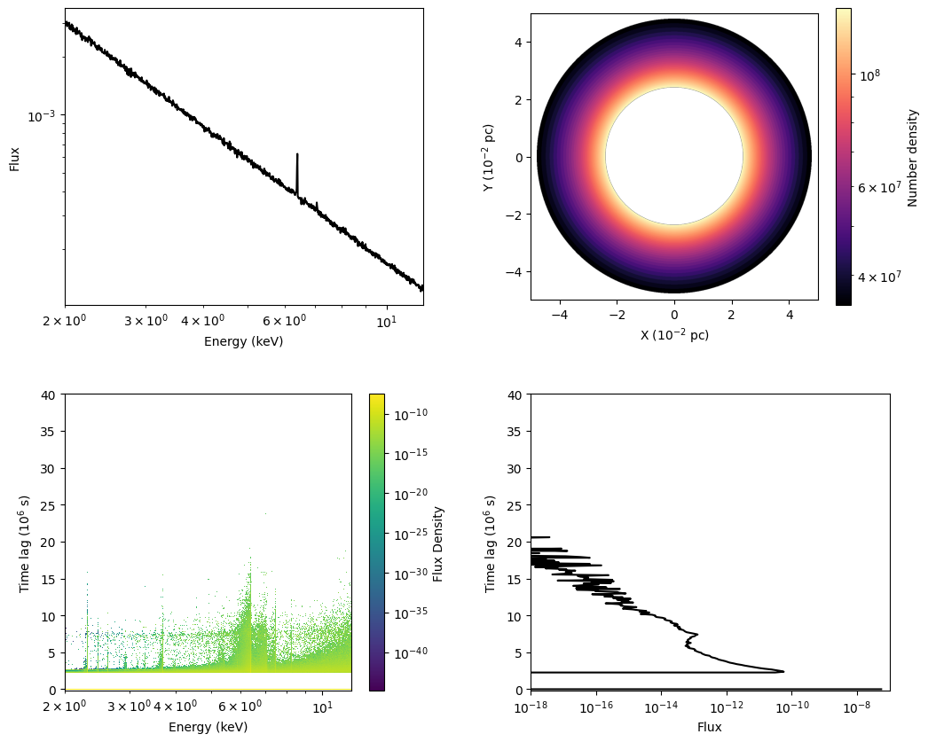
The script generates the figure displayed above, including the following four panels:
Direct emission from the source is shown at a time lag of \(0\), whereas reprocessed emission is shown at time lags \(>0\). The prominent features among the reprocessed emission are fluorescence lines, such as the \(\mathrm{Fe}\;\mathrm{K}\alpha\) line at \(6.4~\mathrm{keV}\). Because the photoelectric absorption cross-section is higher at lower energies, high-energy photons can penetrate and reach the outer regions of the torus. Consequently, these fluorescence lines are produced by the high-energy photons in these outer regions. As a result, the emission of these lines is delayed, exhibiting relatively large time-lag values compared to those of the low-energy reprocessed continuum emission, which is produced predominantly in the inner regions.
The time lag of the \(\mathrm{Fe}\;\mathrm{K}\alpha\) line band relative to the continuum band of the direct emission, measured using the cross-correlation function (CCF), enables reverberation mapping of the surrounding material. First, an intrinsic light curve is assumed. Second, this intrinsic light curve is convolved with the two-dimensional time-lag and energy distribution obtained by SKIRT to produce a mock observed light curve. Third, the mock data are integrated over the fluorescence line energy band and the continuum energy band. Finally, by calculating the CCF between the mock observed light curves of the fluorescence line and the continuum, we obtain a correlation profile that can be directly compared with observations.
Congratulations, you made it to the end of this tutorial!