 |
The SKIRT project
advanced radiative transfer for astrophysics
|
|
The SKIRT project
advanced radiative transfer for astrophysics
|

In this tutorial you will use SKIRT to produce a nearly edge-on V-band image of a dusty disk galaxy model (see illustration above). You will create a ski file containing the appropriate simulation parameters, and then you will actually perform the simulation and review its results. Finally you will adjust the ski file and perform a second simulation with slightly different parameters.
Before starting this tutorial, you should have installed the SKIRT code and preferably PTS as well (see Installation Guide). There are two equivalent ways of creating the ski files for this and other tutorials:
For brevity, the examples in the tutorials omit portions of the SKIRT output, such as the time stamp preceding each line and the version information on the welcome line.
SKIRT stores all parameter values describing a particular simulation in a file with the ".ski" filename extension. To create a new ski file, you need to start SKIRT without any command line arguments. The ski file will be created in the current directory; for this tutorial you could use the run directory you created during SKIRT installation. Enter the following commands in a Terminal window:
$ cd ~/SKIRT/run
$ skirt
If SKIRT is not in your system path, you must replace the last line by the absolute or relative path of the skirt executable; for example:
$ cd ~/SKIRT/run
$ ../release/SKIRT/main/skirt
SKIRT responds with a welcome message and starts an interactive session in the terminal window, during which it will prompt you for all the information describing a particular simulation:
   Welcome to SKIRT v___
   Running on ___ for ___
   Interactively constructing a simulation...
 ? Enter the name of the ski file to be created: MonoDisk
The first question is for the filename of the ski file. For this tutorial, enter "MonoDisk". SKIRT then starts the Q&A sequence that determines the contents of the ski file. In case there is only one possible answer to a particular question, the answer is provided without prompting the user:
   Possible choices for a Monte Carlo simulation:
      1. A Monte Carlo simulation
   Automatically selected the only choice: 1
A ski file always describes a Monte Carlo simulation, so this question is processed automatically.
   Possible choices for the user experience level:
      1. Basic: for beginning users (hides many options)
      2. Regular: for regular users (hides esoteric options)
      3. Expert: for expert users (hides no options)
 ? Enter one of these numbers [1,3] (2): 1
The Q&A session can be tailored to the experience level of the user:
Because this tutorial is intended for beginning users, select Basic level here. Once you are comfortable with the SKIRT configuration process, you can start using Regular level (the default choice).
   Possible choices for the units system:
      1. SI units
      2. Stellar units (length in AU, distance in pc)
      3. Extragalactic units (length in pc, distance in Mpc)
 ? Enter one of these numbers [1,3] (3):
SKIRT offers three sets of input/output units:
Since you will be simulating a galaxy, select extragalactic units (the default choice).
   Possible choices for the output style for wavelengths:
      1. As photon wavelength: λ
      2. As photon frequency: ν
      3. As photon energy: E
 ? Enter one of these numbers [1,3] (1):
There are three options for the output style of the spectral variable: as photon wavelength, frequency, or energy. For example, in the X-ray community one commonly uses the photon energy in keV. For this tutorial, select wavelength (the default choice).
   Possible choices for the output style for flux density and surface brightness:
      1. Neutral: λ F_λ = ν F_ν
      2. Per unit of wavelength: F_λ
      3. Per unit of frequency: F_ν
      4. Counts per unit of energy: F_E
 ? Enter one of these numbers [1,4] (3):
There are four options for the output style of flux-related values, summarized in the following table, using uppercase \(F\) for spatially integrated flux and lowercase \(f\) for surface brightness.
| Style | Quantity | SI units | Stellar & Extragal. units |
| Neutral | \(\lambda F_\lambda = \nu F_\nu\) | \(\mathrm{W}\,\mathrm{m}^{-2}\) | \(\mathrm{W}\,\mathrm{m}^{-2}\) |
| \(\lambda f_\lambda = \nu f_\nu\) | \(\mathrm{W}\,\mathrm{m}^{-2}\,\mathrm{sr}^{-1}\) | \(\mathrm{W}\,\mathrm{m}^{-2}\,\mathrm{arcsec}^{-2}\) | |
| Per unit of wavelength | \(F_\lambda\) | \(\mathrm{W}\,\mathrm{m}^{-3}\) | \(\mathrm{W}\,\mathrm{m}^{-2}\,\mu\mathrm{m}^{-1}\) |
| \(f_\lambda\) | \(\mathrm{W}\,\mathrm{m}^{-3}\,\mathrm{sr}^{-1}\) | \(\mathrm{W}\,\mathrm{m}^{-2}\,\mu\mathrm{m}^{-1}\,\mathrm{arcsec}^{-2}\) | |
| Per unit of frequency | \(F_\nu\) | \(\mathrm{W}\,\mathrm{m}^{-2}\,\mathrm{Hz}^{-1}\) | \(\mathrm{Jy}\) |
| \(f_\nu\) | \(\mathrm{W}\,\mathrm{m}^{-2}\,\mathrm{Hz}^{-1}\,\mathrm{sr}^{-1}\) | \(\mathrm{MJy}\,\mathrm{sr}^{-1}\) | |
| Counts per unit of energy | \(F_\mathrm{E}\) | \(\mathrm{s}^{-1}\,\mathrm{m}^{-2}\,\mathrm{J}^{-1}\) | \(\mathrm{s}^{-1}\,\mathrm{cm}^{-2}\,\mathrm{keV}^{-1}\) |
| \(f_\mathrm{E}\) | \(\mathrm{s}^{-1}\,\mathrm{m}^{-2}\,\mathrm{J}^{-1}\,\mathrm{sr}^{-1}\) | \(\mathrm{s}^{-1}\,\mathrm{cm}^{-2}\,\mathrm{keV}^{-1}\,\mathrm{arcsec}^{-1}\) |
For this tutorial, select per unit of frequency (the default choice) to get surface brightness values in MJy/sr.
   Possible choices for the overall simulation mode:
      1. No medium - oligochromatic regime (a few discrete wavelengths)
      2. Extinction only - oligochromatic regime (a few discrete wavelengths)
      3. No medium (primary sources only)
      4. Extinction only (no secondary emission)
      5. Extinction only with Lyman-alpha line transfer
      6. With secondary emission from dust
      7. With secondary emission from gas
      8. With secondary emission from dust and gas
 ? Enter one of these numbers [1,8] (4): 2
First of all, SKIRT can work in one of two wavelength regimes:
The first two simulation modes in the list above correspond to the oligochromatic wavelength regime; the other modes correspond to the panchromatic wavelength regime. Within these regimes, each simulation mode defines more precisely which overall physical processes will be included in the simulation:
The simulation in this tutorial will calculate the effects of dust extinction at a single wavelength in the V-band, where thermal dust emission has no effect. An oligochromatic simulation is sufficient and most performance-effective for these purposes. Therefore, select the "Extinction only - oligochromatic regime" simulation mode.
? Enter the default number of photon packets launched per simulation segment [0,1e19] (1e6):
The number of photon packets launched during the simulation is a very important parameter, since it determines the level of signal to noise in the results. On the other hand, the simulation run time essentially scales with the number of photon packets. An appropriate number is usually determined experimentally: first run the simulation with a modest number of photon packets, evaluate the results and then run the simulation again with more photon packets if needed.
For your first simulation, leave the number of photon packets at the default value of \(10^6\).
   Possible choices for the source system:
      1. A primary source system
   Automatically selected the only choice: 1
Each SKIRT simulation includes a source system, which holds one or more primary radiation sources. Each of these sources has specific geometric and emission properties which can be configured using built-in features or may be imported from the output of a hydrodynamical simulation in various formats. Since there is only one type of source system, it is automatically selected.
? Enter the wavelengths of photon packets launched from primary sources [1e-6 micron,1e6 micron] (0.55 micron):
For an oligochromatic simulation, the source system requests the list of distinct wavelengths for which to launch photon packets. To obtain an image in the V band, enter a wavelength "list" containing the single value \(\lambda=0.55~\mu{\text{m}}\) (the default value).
   Possible choices for item #1 in the primary sources list:
      1. A primary point source
      2. A primary source with a built-in geometry
      3. A primary source imported from smoothed particle data
         ...
 ? Enter one of these numbers or zero to terminate the list [0,6] (2):
The source system in this tutorial simulation is composed of two components, a stellar disk and a stellar bulge, which are configured using built-in features. So you need to select the "built-in geometry" primary source type (the default value).
   Possible choices for the geometry of the spatial luminosity distribution for the source:
      1. A Plummer geometry
      2. A gamma geometry
         ...
      7. An exponential disk geometry
         ...
     15. A decorator that adds an offset to any geometry
         ...
 ? Enter one of these numbers [1,21] (1): 7
 ? Enter the scale length ]0 pc,∞ pc[: 4000
 ? Enter the scale height ]0 pc,∞ pc[: 350
 ? Enter the radius of the central cavity [0 pc,∞ pc] (0 pc):
Each source component is characterized by a particular spatial geometry. For the stellar disk geometry, select an exponential disk with a scale length of 4 kpc and a scale height of 350 pc, and without a central cavity.
   Possible choices for the spectral energy distribution for the source:
      1. A black-body spectral energy distribution
      2. The spectral energy distribution of the Sun
         ...
 ? Enter one of these numbers [1,9] (1):
 ? Enter the black body temperature ]0 K,∞ K[ (5000 K):
   Possible choices for the type of luminosity normalization for the source:
      1. Source normalization through the integrated luminosity for a given wavelength range
      2. Source normalization through the specific luminosity at a given wavelength
      3. Source normalization through the specific luminosity for a given wavelength band
 ? Enter one of these numbers [1,3] (1): 2
 ? Enter the wavelength at which to provide the specific luminosity [0.0001 micron,1e6 micron]: 0.55
   Possible choices for the luminosity unit style:
      1. Neutral: λ L_λ = ν L_ν
      2. Per unit of wavelength: L_λ
      3. Per unit of frequency: L_ν
      4. Counts per unit of energy: L_E
 ? Enter one of these numbers [1,4] (2):
 ? Enter the specific luminosity at the given wavelength ]0 Lsun/micron,∞ Lsun/micron[: 5e9
Because this tutorial simulation includes just a single wavelength, the emission spectrum of the source does not really matter; we just need to specify the luminosity at that wavelength. However, the Q&A questions handle the general case where both the emission spectrum and some normalization for the luminosity of each source must be specified.
For this tutorial, (arbitrarily) select a black-body spectrum with the default temperature. Then select normalization through the specific luminosity at a given wavelength, with a "per unit of wavelength" luminosity unit style. Finally, specify a luminosity at \(\lambda=0.55~\mu\text{m}\) (the wavelength specified previously) of \(L_\lambda = 5\times10^9~\text{L}_\odot/\mu\text{m}\).
   Possible choices for item #2 in the primary sources list:
      1. A primary point source
      2. A primary source with a built-in geometry
         ...
 ? Enter one of these numbers or zero to terminate the list [0,6] (2):
   Possible choices for the geometry of the spatial luminosity distribution for the source:
         ...
      2. A gamma geometry
      3. A Sérsic geometry
         ...
     18. A decorator that adds a rotation to any geometry
     19. A decorator that constructs a spheroidal variant of any spherical geometry
         ...
 ? Enter one of these numbers [1,23] (1): 19
   Possible choices for the spherical geometry to be made spheroidal:
      1. A Plummer geometry
      2. A gamma geometry
      3. A Sérsic geometry
         ...
 ? Enter one of these numbers [1,6] (1): 3
 ? Enter the effective radius ]0 pc,∞ pc[: 1600
 ? Enter the Sérsic index n ]0.5,10] (1): 2
 ? Enter the flattening parameter q ]0,∞[ (1): 0.7
For the second source component, again select the "built-in geometry" source type. For the geometry, select a spheroidal variant of the Sersic model with effective radius \(R_{\text{e}} = 1.6\) kpc, Sersic index \(n=2\), and flattening parameter \(q=0.7\). SKIRT offers a number of geometry decorators that modify other geometries in various ways, including off-center translation, adding clumpiness, and spheroidal or triaxial flattening. You must select the decorator geometry before the geometry being decorated. Decorator geometries can be nested, for example to form a clumpy triaxial Einasto geometry.
   Possible choices for the spectral energy distribution for the source:
      1. A black-body spectral energy distribution
         ...
 ? Enter one of these numbers [1,9] (1):
 ? Enter the black body temperature ]0 K,∞ K[ (5000 K):
   Possible choices for the type of luminosity normalization for the source:
      1. Source normalization through the integrated luminosity for a given wavelength range
      2. Source normalization through the specific luminosity at a given wavelength
      3. Source normalization through the specific luminosity for a given wavelength band
 ? Enter one of these numbers [1,3] (1): 2
 ? Enter the wavelength at which to provide the specific luminosity [1e-6 micron,1e6 micron]: 0.55
   Possible choices for the luminosity unit style:
      1. Neutral: λ L_λ = ν L_ν
      2. Per unit of wavelength: L_λ
      3. Per unit of frequency: L_ν
      4. Counts per unit of energy: L_E
 ? Enter one of these numbers [1,4] (2):
 ? Enter the specific luminosity at the given wavelength ]0 Lsun/micron,∞ Lsun/micron[: 3e9
Further specify the second source component's luminosity at wavelength \(\lambda=0.55~\mu\text{m}\) as \(L_\lambda = 3\times10^9~\text{L}_\odot/\mu\text{m}\), similar to the procedure used before.
   Possible choices for item #3 in the primary sources list:
      1. A primary point source
      2. A primary source with a built-in geometry
         ...
 ? Enter one of these numbers or zero to terminate the list [0,5] (2): 0
When asked for the third source component, terminate the list by entering zero.
   Possible choices for the medium system:
      1. A medium system
   Automatically selected the only choice: 1
   ...
The medium system contains all the information related to the media in a SKIRT simulation, including:
There is only one type of medium system, so it is automatically selected. Also, when the user experience level is set to Basic, default values are used for all of the extra photon lifecycle options.
   Possible choices for item #1 in the transfer media list:
      1. A transfer medium with a built-in geometry
      2. A transfer medium imported from smoothed particle data
         ...
 ? Enter one of these numbers [1,5] (1):
Similar as for the source system, the medium system can contain a number of medium components (or "media"), each with a specific spatial distribution and material properties. The spatial distribution can be defined through built-in geometries, or it can be loaded from the output of a hydrodynamical simulation. The medium system in this tutorial simulation consists of a single disk of dust, so you need to select a "medium with a built-in geometry" (the default choice).
   Possible choices for the geometry of the spatial density distribution for the medium:
      1. A Plummer geometry
         ...
      7. An exponential disk geometry
         ...
 ? Enter one of these numbers [1,21] (1): 7
 ? Enter the scale length ]0 pc,∞ pc[: 4000
 ? Enter the scale height ]0 pc,∞ pc[: 140
 ? Enter the radius of the central cavity [0 pc,∞ pc[ (0 pc):
For the geometry, select an exponential disk with a scale length of 4 kpc and a scale height of 140 pc, without central cavity. Note that the dust scale height is much smaller than the stellar scale height, which should produce a nice dust lane when viewing the galaxy edge-on.
   Possible choices for the material type and properties throughout the medium:
      1. A typical interstellar dust mix (mean properties)
      2. A THEMIS (Jones et al. 2017) dust mix
         ...
 ? Enter one of these numbers [1,10] (1):
   Possible choices for the type of normalization for the amount of material:
      1. Normalization by defining the total mass
      2. Normalization by defining the total number of entities
      3. Normalization by defining the optical depth along a coordinate axis
         ...
 ? Enter one of these numbers [1,5] (3):
   Possible choices for the axis along which to specify the normalization:
      1. The X axis of the model coordinate sytem
      2. The Y axis of the model coordinate sytem
      3. The Z axis of the model coordinate sytem
 ? Enter one of these numbers [1,3] (3):
 ? Enter the wavelength at which to specify the optical depth [1e-6 micron,1e6 micron]: 0.55
 ? Enter the optical depth along this axis at this wavelength ]0,∞[: 1
In addition to a geometry (determining the spatial distribution), each medium component is characterized by a material mix (determining the optical properties of the medium) and a normalization (determining the total amount of material in the component).
For this tutorial, select a basic dust mixture based on the average properties of the diffuse dust in the Milky Way (the default choice). Further specify a normalization based on a face-on (Z-axis) optical depth of 1 at wavelength \(\lambda=0.55~\mu{\text{m}}\).
  Possible choices for item #2 in the transfer media list:
      1. A transfer medium with a built-in geometry
         ...
 ? Enter one of these numbers or zero to terminate the list [0,5] (1): 0
When asked for the second medium component, terminate the list by entering zero.
   Possible choices for the spatial grid:
      1. A 2D axisymmetric spatial grid in cylindrical coordinates
      2. A 3D spatial grid in cylindrical coordinates
      3. A Cartesian spatial grid
      4. A tree-based spatial grid
 ? Enter one of these numbers [1,4] (1): 1
 ? Enter the inner cylindrical radius of the grid [0 pc,∞ pc[ (0 pc):
 ? Enter the outer cylindrical radius of the grid ]0 pc,∞ pc[: 20000
 ? Enter the start point of the cylinder in the Z direction [-∞ pc,∞ pc]: -5000
 ? Enter the end point of the cylinder in the Z direction [-∞ pc,∞ pc]: 5000
   Possible choices for the bin distribution in the radial direction:
      1. A linear mesh
      2. A power-law mesh
      3. A symmetric power-law mesh
      4. A logarithmic mesh
 ? Enter one of these numbers [1,4] (1): 2
 ? Enter the number of bins in the mesh [1,100000] (100): 100
 ? Enter the bin width ratio between the last and the first bin ]0,∞[ (1): 20
   Possible choices for the bin distribution in the Z direction:
      1. A linear mesh
      2. A power-law mesh
      3. A symmetric power-law mesh
 ? Enter one of these numbers [1,3] (1): 3
 ? Enter the number of bins in the mesh [1,100000] (100): 100
 ? Enter the bin width ratio between the outermost and the innermost bins ]0,∞[ (1): 30
As mentioned above, SKIRT discretizes the spatial domain on a grid, i.e. a collection of small cells covering three-dimensional space. Within each cell, the density of the medium and quantities such as the radiation field are considered to be uniform. SKIRT offers several types of spatial grids, which can be selected depending on the requirements of the simulation. Depending on the symmetries in the source and medium distributions, SKIRT supports 1D spherical grids (the grid cells are thin concentric shells), 2D axisymmetric grids (the grid cells have the form of a torus), 3D cartesian grids (the grid cells are little cuboids), and unstructured Voronoi grids (each cell is a convex polyhedron). Simulations in a 1D or 2D grid, when allowed by the system's symmetries, are much more efficient than simulations in a full 3D grid.
Each grid type features parameters to set the detailed grid cell distribution in each direction. This is one of the most difficult tasks during model setup. The grid must be chosen in such a way that the entire configuration space is covered and with the resolution highest in those parts where the medium density is highest or the radiation field changes most. In many cases, a linear distribution is not the best choice. A logarithmic grid is denser in the center than in the outer regions, which is often required. A logarithmic grid however, has the drawback that it does not go all the way down to zero. A useful alternative is the power-law grid, in which the spatial cells are also gradually bigger when they are farther away from the center.
For this tutorial simulation, select a 2D axisymmetric grid in cylindrical coordinates with a power-law mesh in the radial direction and a symmetric power-law mesh in the vertical direction. Choosing a symmetric vertical mesh ensures that the grid cells are small in the center of the mesh and larger to the top and bottom of the mesh. The radial mesh is symmetric relative to the origin by definition. Here we want the grid cells to be small near \(R=0\), i.e. at the lower coordinate of the mesh. Specify a grid radius of 20 kpc and grid height of 10 kpc centered on the origin. This grid size should be sufficient to contain the vast majority of the dust in the exponential disk configured earlier. Specify 100 cells in each direction, so that there are 10000 cylindrical cells in total. Further specify a ratio of the width of the outermost to the innermost bin of 20 in the radial and 30 in the vertical direction; the ratio is somewhat larger in the vertical direction because we want a higher resolution there in the inner regions.
   Possible choices for the instrument system:
      1. An instrument system
   Automatically selected the only choice: 1
Running a radiative transfer simulation is not particularly useful unless the results are registered by one or more instruments, which collect the photon packets that leave the system, in a process similar to the operation of real instruments at a telescope.
The SKIRT instruments essentially emulate imaging spectrometers, i.e. 3D spectrographs with one wavelength dimension (determined by the simulation's wavelength grid) and two spatial directions on the plane of the sky. Each instrument is characterized by its own frame properties (pixel size and field of view) and by its position with respect to the system (for axisymmetric systems, this means the inclination and distance).
The instrument system contains one or more instruments. It should be noted that the number of instruments, and the pixel size of these instruments, influence both memory consumption (for storing the data cubes) and simulation run time (for peeling off photon packets in the direction of each instrument).
There is only one type of instrument system (simply a list of instruments) so the default choice is automatically selected.
   Possible choices for item #1 in the instruments list:
      1. A distant instrument that outputs the spatially integrated flux density as an SED
      2. A distant instrument that outputs the surface brightness in every pixel as a data cube
      3. A distant instrument that outputs both the flux density (SED) and surface brightness (data cube)
 ? Enter one of these numbers or zero to terminate the list [0,3] (1): 2
 ? Enter the name for this instrument: i88
 ? Enter the distance to the system ]0 Mpc,∞ Mpc[: 10
 ? Enter the inclination angle θ of the detector [0 deg,180 deg] (0 deg): 88
 ? Enter the total field of view in the horizontal direction ]0 pc,∞ pc[: 40000
 ? Enter the number of pixels in the horizontal direction [1,10000] (250): 800
 ? Enter the total field of view in the vertical direction ]0 pc,∞ pc[: 10000
 ? Enter the number of pixels in the vertical direction [1,10000] (250): 200
 ? Do you want to record flux components separately? [yes/no] (no):
For the first (and only) instrument in this tutorial simulation, select a distant instrument that outputs the surface brightness in every pixel. Since you will be shooting photon packets at a single wavelength only, the "data cube" will have only one frame, and it doesn't make much sense to produce a spectrum.
Specify an appropriate name for the instrument. This name is used to identify the output files for the instrument. This is not so relevant here, but it becomes important when there are multiple instruments. Further specify a size of 800 times 200 pixels with a scale of 50 pc, a distance of 10 Mpc from the galaxy, and an inclination of 88 degrees. You don't need to turn on the option to record flux components separately.
   Possible choices for item #2 in the instruments list:
      1. A distant instrument that outputs the spatially integrated flux density as an SED
         ...
 ? Enter one of these numbers or zero to terminate the list [0,3] (1): 0
When asked for the second instrument, enter zero to terminate the list.
   Possible choices for the probe system:
      1. A probe system
   Automatically selected the only choice: 1
SKIRT offers two kinds of output. Most importantly, at the end of the simulation run, the instruments described in the previous section output "mock observations", i.e. fluxes obtained by detecting photon packages during the simulation. This kind of output is usually the main simulation result.
It is, however, often meaningful to also output information on data structures constructed in preparation for or during the simulation run. This may include internal diagnostics (such as a list of coordinates that allow plotting the spatial grid), and it may include physical quantities that are computed by the simulation but cannot be "observed" from the outside, such as the local radiation field throughout the spatial domain. This kind of output is produced by a separate set of objects, called "probes".
Depending on a probe's type, it is invoked at one of two points in the simulation run to produce its output: at the end of the setup phase, or at the very end of the simulation run. Each probe has a name, serving to unambiguously distinguish its output files, and some probe types offer additional options. It possible and often useful to include differently configured multiple probes of the same type.
All probes are part of the probe system. Because there is only one type of probe system, it is selected automatically.
   Possible choices for item #1 in the probes list:
      1. Convergence: information on the spatial grid
      2. Convergence: cuts of the medium density along the coordinate planes
      3. Source: luminosities of primary sources
      4. Internal spatial grid: density of the medium
      5. Internal spatial grid: opacity of the medium
      6. Properties: basic info for each spatial cell
      7. Properties: data files for plotting the structure of the grid
      8. Properties: aggregate optical material properties for each medium
 ? Enter one of these numbers or zero to terminate the list [0,8] (1): 1
 ? Enter the name for this probe: cnv
 ? Enter the wavelength at which to determine the optical depth [1e-6 micron,1e6 micron] (0.55 micron):

   Possible choices for item #2 in the probes list:
         ...
      2. Convergence: cuts of the medium density along the coordinate planes
         ...
   ? Enter one of these numbers or zero to terminate the list [0,8] (1): 2
   ? Enter the name for this probe: cut

   Possible choices for item #3 in the probes list:
         ...
      7. Properties: data files for plotting the structure of the grid
         ...
 ? Enter one of these numbers or zero to terminate the list [0,8] (1): 7
 ? Enter the name for this probe: grid

   Possible choices for item #4 in the probes list:
         ...
      8. Properties: aggregate optical material properties for each medium
 ? Enter one of these numbers or zero to terminate the list [0,8] (1): 8
 ? Enter the name for this probe: opt
   Possible choices for item #5 in the probes list:
      1. Convergence: information on the spatial grid
         ...
 ? Enter one of these numbers or zero to terminate the list [0,8] (1): 0
Configure the following four probes, in arbitrary order, and specify their names as follows.
| Probe type | Probe name |
|---|---|
| Convergence: information on the spatial grid | cnv |
| Convergence: cuts of the medium density along the coordinate planes | cut |
| Properties: data files for plotting the structure of the grid | grid |
| Properties: aggregate optical material properties for each medium | opt |
Finally, when asked for the subsequent probe, enter zero to terminate the list.
   Successfully created ski file 'MonoDisk.ski'.
   To run the simulation use the command: skirt MonoDisk
After all questions have been answered, SKIRT writes out the resulting ski file and exits.
To actually run the simulation, enter the following command (with the same current directory):
$ skirt MonoDisk
Or if SKIRT is not in your system path, include the absolute or relative path of the skirt executable; for example:
$ ../release/SKIRT/main/skirt MonoDisk
SKIRT responds with a welcome message and immediately starts performing the simulation. In this mode SKIRT never asks a question so it can be left to run unattended:
   Welcome to SKIRT v___
   Running on ___ for ___
   Constructing a simulation from ski file 'MonoDisk.ski'...
   Starting simulation MonoDisk using __ threads and a single process...
   Starting setup...
     Oligochromatic wavelength regime
     With transfer medium
     Model and grid symmetry: 2D
   ...
 - Finished simulation MonoDisk using __ threads and a single process in __ s.
   Available memory: 16 GB -- Peak memory usage: 24.7 MB (0.2%)
SKIRT produces various log messages to report on specific activities and overall progress. The execution of a simulation progresses in several distinct stages:
The output files for this tutorial simulation are written in the current directory. All filenames start with "MonoDisk", i.e. the name of the ski file. Two files are always generated for every simulation:
MonoDisk_log.txt contains the progress log as it was written to the console.MonoDisk_parameters.xml contains a copy of the ski file, with a time stamp of when the simulation was run.During the setup output stage, the probes configured for this tutorial simulation generated the following files:
MonoDisk_cnv_convergence.dat is a short text file providing a consistency check on the spatial grid. It lists the total dust mass as well as the optical depth of the dust along each of the coordinate axes (a) as expected from the input configuration and (b) obtained by integrating over the spatial grid after discretizing the dust distribution. If these numbers match within a few percent, the spatial grid samples the dust density well. If there are large deviations, it might be useful to consider a different grid cell distribution (e.g. with a larger extent, with more resolution, or with more or less contrast between inner and outer cells).MonoDisk_opt_opticalprops_0.dat lists various aggregate optical properties (such as absorption and scattering cross sections) of the material mix used in the simulation at the single oligochromatic wavelength configured for the simulation. The number in the filename indicates the zero-based index of the medium component to which the properties correspond. In this tutorial simulation, there is only a single medium component so there is only one file.MonoDisk_cut_dust_t_xy.fits & MonoDisk_cut_dust_t_xz.fits (t for "theorical") are single-frame FITS data files, each providing a 1024 x 1024 pixel map of the theoretical dust density in a coordinate plane, across the total extent of the spatial grid. These density values are determined from the medium distribution as if there is an infinitely fine spatial grid.MonoDisk_cut_dust_g_xy.fits & MonoDisk_cut_dust_g_xz.fits (g for "gridded") are single-frame FITS data files, each providing a 1024 x 1024 pixel map of the grid-discretized dust density in a coordinate plane, across the total extent of the spatial grid. These density values are read from the finite-resolution spatial grid constructed for the simulation.MonoDisk_grid_grid_xy.dat & MonoDisk_grid_grid_xz.dat are data files in a text format that can be easily plotted. Each file describes the intersection of the spatial grid with one of the coordinate planes.During the final output stage, the instrument configured for this tutorial simulation also produces an output file:
MonoDisk_i88_total.fits (where "i88" is the specified instrument name) is a FITS file containing the data cube with the total surface brightness for each pixel as detected by the instrument. Since the simulation has only one wavelength, there is only a single frame in the output file.With few exceptions, SKIRT produces data (mock observables and diagnostic information) in two formats:
ASCII text files can be viewed using any text editor and can easily be processed by many software tools. FITS files can be viewed with a dedicated FITS viewer such as SAOImage DS9, which you may want to install as described in the Installation Guide.
The Python language ecosystem also has extensive support for both data formats. The almost standard Python package numpy supports reading text column files into numpy arrays, and the well-known astronomy Python package astropy supports reading FITS data into numpy arrays. Once in memory, these data can be further processed at will.
Based on these packages, the Python toolkit for SKIRT (PTS) offers functions to read SKIRT output files with some extra intelligence (e.g., interpreting units), and it offers high-level commands to rapidly visualize some specific SKIRT output. In the following subsections, you will use some of the high-level PTS commands to visualize results of the simulation configured and performed in this tutorial.
It is often instructive to compare the theoretical and gridded dust density cuts produced by the probe configured as "cut" in this simulation. PTS offers a convenient way to do this. With the simulation results residing in the current directory, enter the following command:
$ pts plot_convergence .
The dot at the end tells the command to look for simulation results in the current directory. The command name can be shortened to its first portion (e.g. "plot_conv") as long as the shorthand defines a unique command name. PTS should respond with a message indicating that a PDF file named MonoDisk_cut_dust.pdf has been created.
Open this file in a PDF viewer; it should look similar to the example below:
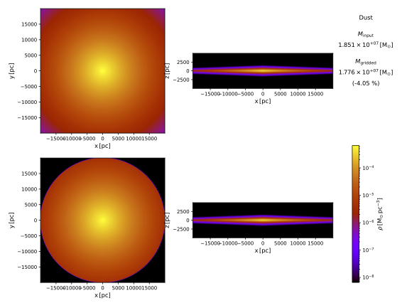
The top row shows horizontal and vertical cuts through the theoretical dust density, and the bottom row shows the corresponding cuts through the gridded dust density. This is very obvious for the gridded horizontal cut, which is cut off at the extent of the cylindrical grid. When you look closely or zoom in on the PDF, the cellular structure of the gridded cut becomes apparent, although it is hard to see in this example.
Similarly, PTS offers a command for plotting the spatial grid structure used in a SKIRT simulation. Again with the SKIRT output directory as your current directory, enter the command (be sure to include the dot at the end):
$ pts plot_grids .
PTS now creates the files MonoDisk_grid_grid_xy.pdf and MonoDisk_grid_grid_xz.pdf. Open these files in a PDF viewer. Compare the grid structure to the cellular structure of the gridded density cuts plotted in the previous subsection.
Finally, you want to have a look at the actual simulation result, i.e. the surface brightness detected and output by the instrument in your simulation. An excellent option is to open the MonoDisk_i88_total.fits file in an interactive FITS viewer. If the viewer allows it, set the scale for displaying the pixel values to logarithmic.
Alternatively, PTS offers a command to create a regular RGB image in PNG format for the FITS files generated by SKIRT instruments. By default PTS uses the first FITS frame for the Blue channel, the last FITS frame for the Red channel, and some frame in the middle for the Green channel. Because this tutorial simulation is monochromatic, all three frames are identical so that the result is actually a grayscale image.
Again with the SKIRT output directory as your current directory, enter the command (be sure to include the dot at the end):
$ pts make_images .
PTS now creates the file MonoDisk_i88_total.png. Open this file with an image viewer. It should look similar to the image at the start of this tutorial (see Monochromatic simulation of a dusty disk galaxy), except that your image shows substantially more noise than the image shown as part of this tutorial. Improving the signal-to-noise ratio for the results of a SKIRT simulation is conceptually simple: shoot (many) more photon packets...
There is no need to go through the lengthy interactive Q&A process again if you just want to re-run a simulation with slightly adjusted parameters. You can manually edit the ski file instead. Duplicate the file MonoDisk.ski to a new file named MonoDisk2.ski and open this new file in any decent text editor. It should look similar to the following snippet, where "..." indicates omitted information:
...
<skirt-simulation-hierarchy type="MonteCarloSimulation" ...>
    <MonteCarloSimulation userLevel="Basic" simulationMode="OligoExtinctionOnly" ... numPackets="1e6">
        ...
        <sourceSystem type="SourceSystem">
            ...
        </sourceSystem>
        <mediumSystem type="MediumSystem">
            ...
        </mediumSystem>
        <instrumentSystem type="InstrumentSystem">
            <InstrumentSystem>
                <instruments type="Instrument">
                    <FrameInstrument instrumentName="i88" distance="10 Mpc"
                            inclination="88 deg" azimuth="0 deg" roll="0 deg"
                            fieldOfViewX="4e4 pc" numPixelsX="800" centerX="0 pc"
                            fieldOfViewY="1e4 pc" numPixelsY="200" centerY="0 pc"
                            recordComponents="false" numScatteringLevels="0"
                            recordPolarization="false" recordStatistics="false"/>
                </instruments>
            </InstrumentSystem>
        </instrumentSystem>
        <probeSystem type="ProbeSystem">
            ...
        </probeSystem>
    </MonteCarloSimulation>
</skirt-simulation-hierarchy>
Make the following changes:
Save your changes and execute the adjusted simulation using the command "skirt MonoDisk2". The simulation will run substantially slower because it is launching more photon packets and because there are more instruments.
Look at the differences between output files:
MonoDisk_i88_total.fits and MonoDisk2_i88_total.fits (more photon packets)MonoDisk2_i84_total.fits and MonoDisk2_i88_total.fits (different inclination)Congratulations, you made it to the end of this tutorial!