Nonzero redshift & CMB dust heating

Introduction

SKIRT allows explicitly configuring and simulating astrophysical objects at non-zero redshift. In addition to actually shifting the wavelengths in the recorded synthetic observations, this enables SKIRT to perform the appropriate relativistic flux and surface brightness calibrations and to simulate the effect of the cosmic microwave background on the dust temperature.

This topic summarizes the related configuration options, physical mechanisms, and numerical recipes. The discussion is organized in sections as follows:

• Redshift and cosmology
• Instruments and calibration
• Dust heating by the CMB

Redshift and cosmology

SKIRT assumes that the complete simulated model (or, more precisely, the model coordinate frame) is at a single, given redshift $z$ within the range $0\le z\le 15$, i.e. including the epoch of reionization. The MonteCarloSimulation class offers the cosmology property for specifying the cosmology related parameters of the input model in addition to the redshift. The cosmology property simply points to an instance of a Cosmology subclass. The current implementation provides the following two Cosmology subclasses:

Class name	Description	Properties
LocalUniverseCosmology	The model is in the Local Universe at redshift zero	None
FlatUniverseCosmology	The model is at some nonzero redshift in a flat universe	$z,h,{\mathrm{\Omega }}_{\mathrm{m}}$

LocalUniverseCosmology is the default "cosmology" and reproduces "Local Universe" behavior at redshift zero. On the other hand, FlatUniverseCosmology specifies a standard spatially-flat $\mathrm{\Lambda }\mathrm{C}\mathrm{D}\mathrm{M}$ cosmology model. In addition to the redshift, this cosmology has two parameters, namely the reduced Hubble constant $h=H_0/(100\mathrm{k}\mathrm{m}{\mathrm{s}}^{-1}{\mathrm{M}\mathrm{p}\mathrm{c}}^{-1})$ and the matter density fraction ${\mathrm{\Omega }}_{\mathrm{m}}$. These are summarized in the following table. The default values are compatible with recent observations (Planck 2018) and close to the values used by many recent cosmological simulations. If $z=0$, the behavior is the same as that of a LocalUniverseCosmology.

Property	Description	Default
redshift	Redshift $0\le z\le 15$ of the model coordinate frame	$z=1$
reducedHubbleConstant	Reduced Hubble constant $h$	$h=0.675$
matterDensityFraction	Cosmological matter density fraction ${\mathrm{\Omega }}_{\mathrm{m}}$	${\mathrm{\Omega }}_{\mathrm{m}}=0.310$

Instruments and calibration

Distant instruments

Instruments using parallel projection are implemented by DistantInstrument subclasses and include instances of SEDInstrument, FrameInstrument, and FullInstrument. If the model redshift is non-zero, a distant instrument can be placed in either the model rest-frame (at a given distance) or the observer frame (honoring the redshift). To allow this selection, the DistantInstrument class allows its distance property to have a zero value. Specifically,

• If distance is non-zero, the instrument is placed in the rest frame of the model at the given (non-relativistic) distance. Wavelengths are not shifted and fluxes are calibrated as usual.
• If distance is zero, the instrument is placed in an observer frame corresponding to the redshift specified for the model. The wavelength of each detected photon packet is shifted accordingly before the packet's contribution is recorded in the instrument, and flux/surface brightness calibration takes into account the relevant relativistic effects including the luminosity distance.
• If distance is zero and the model redshift is zero as well, a fatal error is issued during setup.

This approach allows the on-the-fly convolution for a broadband-based instrument to occur in either the rest frame or the observer frame depending on the instrument's settings. A configuration might even include both type of instruments at the same time.

Local instruments

The other SKIRT instruments include instances of AllSkyInstrument and PerspectiveInstrument. These instruments are "local" in the sense that they are commonly positioned inside or very near the input model. As a consequence, these instruments are always considered to be in the rest frame of the input model.

Calibration

We consider the calibration for a distant instrument assuming a standard spatially-flat $\mathrm{\Lambda }\mathrm{C}\mathrm{D}\mathrm{M}$ cosmology. This means that the line-of-sight and transverse comoving distances are identical. We further ignore the radiation density, which is justified for the allowed redshift range $z\le 15$. With these assumptions, the comoving distance $d_{\mathrm{M}}(z)$ corresponding to redshift $z$ can be obtained from the matter density fraction ${\mathrm{\Omega }}_{\mathrm{m}}$ and the Hubble constant $H_0=h\times 100\mathrm{k}\mathrm{m}{\mathrm{s}}^{-1}{\mathrm{M}\mathrm{p}\mathrm{c}}^{-1}$ using

$$d_{\mathrm{M}}(z)=\frac{c}{H_0}{\int }_0^z\frac{\mathrm{d}{z}^{\prime }}{\sqrt{{\mathrm{\Omega }}_{\mathrm{m}}(1+z^{\prime }{)}^3+(1-{\mathrm{\Omega }}_{\mathrm{m}})}}$$

where $c$ is the speed of light. The integral can easily be evaluated numerically. Because this evaluation happens just once during setup, speed is not important and there is no need to use more complicated methods.

The angular-diameter distance $d_{\mathrm{A}}(z)$ and the luminosity distance $d_{\mathrm{L}}(z)$ are then obtained from

$$d_{\mathrm{A}}(z)=(1+z{)}^{-1}{d}_{\mathrm{M}}(z)$$

and

$$d_{\mathrm{L}}(z)=(1+z)d_{\mathrm{M}}(z).$$

The angular-diameter distance converts a proper transverse separation $\mathrm{d}l$ to the corresponding observed angular separation $\mathrm{d}\psi$,

$$\mathrm{d}\psi =\frac{\mathrm{d}l}{d_{\mathrm{A}}(z)}.$$

This is used for surface brightness calibration and to properly calculate the angular pixel size, which is written to the FITS file header representing the instrument data cube.

The luminosity distance converts a total luminosity $L_{\mathrm{t}\mathrm{o}\mathrm{t}}$ to the corresponding observed total flux $F_{\mathrm{t}\mathrm{o}\mathrm{t}}$,

$$F_{\mathrm{t}\mathrm{o}\mathrm{t}}=\frac{L_{\mathrm{t}\mathrm{o}\mathrm{t}}}{4\pi d_{\mathrm{L}}^2(z)}$$

or a neutral-style monochromatic luminosity $\lambda L_{\lambda }$ to the corresponding observed neutral-style flux,

$$(1+z)\lambda F_{\lambda }[(1+z)\lambda ]=\frac{\lambda L_{\lambda }[\lambda ]}{4\pi d_{\mathrm{L}}^2(z)}$$

where $\lambda$ is the emitted wavelength and $(1+z)\lambda$ is the observed wavelength. This is used for both flux density and surface brightness calibration.

Dust heating by the CMB

The temperature of the cosmic microwave background (CMB) increases with redshift. Therefore, at higher redshifts, the CMB radiation may contribute significantly to the heating of cold dust grains. To allow including this effect in SKIRT dust heating and emission calculations, the DustEmissionOptions class offers a Boolean property called includeHeatingByCMB. This property is available even for models at redshift zero, although in that case CMB heating will be insignificant except for very contrived simulation models.

If CMB dust heating is turned on in the configuration, rather than performing actual radiative transfer for the CMB radiation, the dust heating/emission calculations in the EquilibriumDustEmissionCalculator and StochasticDustEmissionCalculator classes include an additional source term corresponding to the CMB spectrum. The extra radiation field for a model at redshift $z$ is given by

$$B_{\lambda }(\lambda ,[1+z]T_{\mathrm{C}\mathrm{M}\mathrm{B}}^{z=0})\mathrm{w}\mathrm{i}\mathrm{t}\mathrm{h}{T}_{\mathrm{C}\mathrm{M}\mathrm{B}}^{z=0}=2.725\mathrm{K}$$

where $B_{\lambda }(\lambda ,T)$ is the Planck function. The dust emission calculators pre-calculate and add this spectrum to the radiation field $J_{\lambda }(\lambda )$ provided for each calculation.

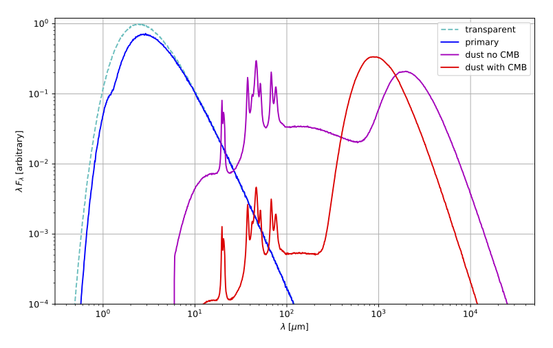
Implementing CMB dust heating as a "forced" source term in the dust heating calculations has some implications worth considering. An important benefit is that the mechanism consumes a trivial amount of memory and processing time. On the other hand, it assumes that the opacity of the medium at CMB wavelengths is sufficiently low for the CMB to be homogeneous across the spatial domain. Taking into account the actual opacity of the medium would require performing a full radiative transfer simulation (i.e., shooting photon packets through the medium). And lastly, while the effects of the CMB radiation on the dust emission are included, the CMB radiation itself never reaches the instruments. In other words, the "observed" fluxes do not include the CMB background itself, just its effects on the dust emission spectrum.

The figure below illustrates the effect of enabling dust heating by the CMB for a toy model including a central point source in spherical dust cloud placed at redshift 5. The model specifies the Themis dust mix and employs stochastic dust heating. The average dust temperature is about 8 K when CMB heating is disabled, and about 16 K when it is enabled. The unrealistically low dust temperature of course magnifies the effect of the CMB heating.