This page describes SKIRT's capabilities for obtaining reliability statistics (a form of "error bars") for the fluxes generated by the instruments in the simulation.

Background and objectives

A SKIRT simulation discretizes all relevant physical quantities along spatial and spectral dimensions and represents the flow of radiative energy using a finite number of photon packets. These numerical approximations necessarily affect the simulation results. A common method to get a handle on these inaccuracies is to perform a series of convergence tests, verifying that the results are stable for increasing discretization resolution.

Moreover, the Monte Carlo radiative transfer method employed by SKIRT inherently introduces noise in the simulation results. The various acceleration and variance reduction techniques make it impossible to precisely predict these noise levels across the spatial and/or spectral dimension. While convergence tests remain an important tool to verify overall robustness, sometimes one requires a more quantitative analysis of the noise levels for a given simulation result, such as the individual pixels in an image. This can be achieved using the optional statistics output by the SKIRT instruments.

The treatment below is based on the discussion in the Overview and Theory manual for MCNP, a Monte Carlo N-Particle transport code developed by Los Alamos National Laboratory in the United States. For more information, see Camps and Baes 2018, Camps and Baes 2020, and references therein.

Statistical metrics

A SKIRT instrument defines a set of bins that each record flux contributions in a specific spatial and spectral interval. The total simulation result for a given bin is obtained by accumulating the contributions $w_{i}$ of individual photon packets, i.e. $\sum_{i} w_{i}$ , where the index $i$ and the sum run over the $N$ photon packets launched during the simulation. All contributions to the same bin from the complete emission and scattering history of a given photon packet are aggregated into a single contribution $w_{i}$ . If statistics are requested, the instrument tracks the sums $W_{k} = \sum_{i} w_{i}^{k}$ for $k = 0, 1, 2, 3, 4$ during the simulation (as opposed to just the sum for $k = 1$ ) and outputs these data alongside the regular results. The sum $W_{0}$ yields the number of photon packet contributions to the given bin, which by itself may be an interesting value. Using the higher order sums one can obtain more important statistical metrics.

Foremost, the relative error, $R$ , is given by

$R = {[\frac{W_{2}}{W_{1}^{2}} - \frac{1}{N}]}^{1 / 2} .$

The relative error $R$ should be smaller than 0.1 for the corresponding result to be considered reliable. In that case, $R$ can indeed be interpreted as a relative error on the result. In the range $0.1 < R < 0.2$ , however, results are questionable, and for $R > 0.2$ , results are unreliable.

The variance of the variance, VOV, is a higher-order statistic given by

$V O V = \frac{W_{4} - 4 W_{1} W_{3} / N + 8 W_{2} W_{1}^{2} / N^{2} - 4 W_{1}^{4} / N^{3} - W_{2}^{2} / N}{{[W_{2} - W_{1}^{2} / N]}^{2}} .$

The VOV measures the statistical uncertainty in the value for $R$ . It is much more sensitive to large fluctuations in the $w_{i}$ values than is $R$ , and it can thus detect situations where the obtained $R$ value is unreliable. The value of the VOV should be below 0.1 to ensure a reliable confidence interval.

Another useful quantity is the figure of merit, FOM, defined as

$F O M = \frac{1}{R^{2} T},$

where $T$ is the computer time spent on the simulation in seconds. Because the computer time is roughly proportional to the number of photon packets $N$ and the square of the relative error should scale more or less as $1 / N$ (for large $N$ ), the FOM should be approximately constant once the solution has converged. The evolution of the FOM for increasing $N$ can thus be used as a reliability indicator. The FOM also provides a measure for the efficiency or ‘merit’ of a particular method for solving the problem at hand. A higher FOM indicates that the simulation can reach a given noise level in less computer time.

Configuration

Tracking and outputting statistics can be enabled for any SKIRT instrument individually by setting its recordStatistics property to true. As indicated above, the output includes the sums $W_{k} = \sum_{i} w_{i}^{k}$ ( $k = 0, 1, 2, 3, 4$ ) for each instrument bin, from which one can easily calculate the corresponding values for the $R$ and VOV metrics. Keep in mind that gathering and storing this extra information uses both memory and processing time.

To obtain the correct metrics, it is important to configure the instrument with the precise spatial and spectral resolution of interest. Specifically, rebinning (combining the data for two or more adjacent bins) after the fact does not yield the correct metrics. This is so because multiple contributions caused by a given photon packet that happen to arrive in a particular bin cannot be considered statistically independent and thus must be (and are) aggregated into a single $w_{i}$ value. This can happen, for example, when a packet scatters multiple times in the line-of-sight of the bin. This aggregation issue is irrelevant for a regular flux calculation, corresponding to the first order sum $W_{1}$ , because the contributions are added linearly. However, the aggregation does matter for the higher order sums, which are nonlinear expressions of the individual contributions.

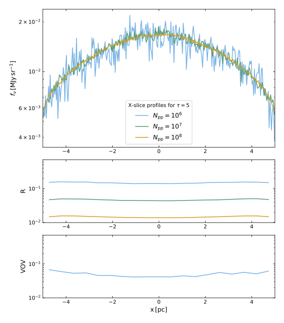
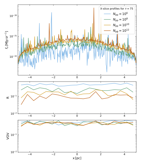
Example: radiation penetrating thick slab

A very informative, albeit somewhat theoretical, application of SKIRT's statistical metrics is provided by Camps and Baes 2020. The SKIRT simulation in this example includes a cuboidal slab of material illuminated by a monochromatic point source. The distant (parallel-projected) instrument on the opposite side covers a slice across the length of the slab and is offset from the center so that the point source is not in the field of view. Each pixel in the instrument frame spans the full width of the slice, causing all photon packet contributions along the width of the slice to end up in the same pixel, and the set of pixels to form a linear sequence of thin rectangles along the length of the slice. The figure below shows the flux density profile detected by this instrument for a varying total number of photon packets $N_{p p}$ launched during the simulation (top row) and the corresponding values of the relative error $R$ (middle row) and the variance of the variance VOV (bottom row).

The left panel illustrates that for an optical depth across the slab of $τ = 5$ the results are essentially converged starting at $N_{p p} \geq 10^{7}$ . In this case, $R < 0.1$ and the value of the VOV is below $10^{- 2}$ (which is why the corresponding curves are missing), so that both $R$ and the actual simulation results can be deemed reliable. The situation shown in the right panel for an optical depth of $τ = 75$ is totally different. The average flux density rises significantly with an increasing number of photon packets, which is a strong indication that something fishy is going on. The good news is that we can now use statistical analysis to evaluate the results. It appears that $R$ (finally) dips under the reliability threshold for $N_{p p} = 10^{12}$ . However, the VOV is still well above the threshold, so the value of $R$ cannot really be trusted. This is reflected by two features apparent in the flux density profiles. Firstly, extrapolation of the progression of the flux profile average with increasing $N_{p p}$ seems to indicate room for a further increase. Secondly, the flux density curve shows several large peaks of an order of magnitude or more even for the simulation with $N_{p p} = 10^{12}$ . We can conclude from this analysis that the results are still not fully converged.

The simulation with $N_{p p} = 10^{12}$ shown in the right panel ran for over 6 hours on a 24-core server. Calculating the next step in the progression, i.e. $N_{p p} = 10^{14}$ , would take 25 days on the same machine. While using a larger, multi-node computer system could shorten the elapsed time, there is no guarantee of convergence. In fact, the lack of progression of the VOV values up to $N_{p p} = 10^{12}$ seems to indicate that one would need to process several orders of magnitude more photon packets for the results to be converged with an acceptable signal to noise ratio.

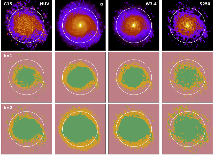
Example: high-resolution synthetic galaxy images

A more practical application of SKIRT's statistical metrics is provided by Camps et al. 2022. These authors produce high-resolution synthetic UV–submm images for Milky Way-mass simulated galaxies from the ARTEMIS project. To evaluate convergence on a pixel by pixel basis, they calculate the relative error $R$ for each pixel in a representative set of broadband images at selected viewing angles. The figure below shows these statistics for the face-on view of a representative ARTEMIS galaxy in four selected bands from UV to submm wavelengths.

The synthetic surface brightness maps in the top row use a logarithmic colour scale; the transition between red and blue marks 1/100 of the maximum surface brightness. Each of the underlying data frames has $1728^{2}$ $50 \times 50$ pc pixels, corresponding to the 86 kpc field of view. The second row ( $b = 1$ ) shows the corresponding $R$ value for each of these pixels indicating reliable ( $R < 0.1$ , green), questionable ( $0.1 < R < 0.2$ , orange) and unreliable ( $R > 0.2$ , red) image areas. The third row ( $b = 2$ ) shows the same statistic after $2 \times 2$ binning into $100 \times 100$ pc pixels. As expected, this binning results in a substantial increase in reliability at the cost of lower resolution.

At the binned $b = 2$ level, the reliable area (green) essentially covers all pixels with a value down to 1/100 of the maximum surface brightness (yellow and red). At the original $b = 1$ level, one needs to include the questionable area (orange) to achieve a similar coverage. Generally, the FUV/NUV bands tend to show somewhat poorer statistics because of the relatively lower fluxes and higher extinction involved in that wavelength range.