Expanding or contracting Lyman-alpha sphere

Introduction

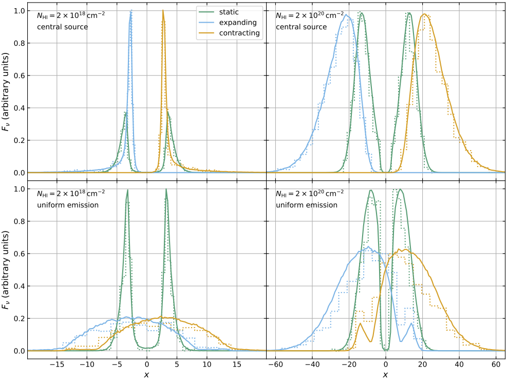
Tasitsiomi 2006 presents numerical solutions for the spectrum emerging from static, expanding, or contracting neutral hydrogen spheres with an embedded Lyman-alpha source. All models include a uniform neutral hydrogen sphere at a temperature of $T=2\times {10}^4$ K and with a radial number column density of $N_{\mathrm{H}\mathrm{I}}=2\times {10}^{18}{\mathrm{c}\mathrm{m}}^{-2}$ or $N_{\mathrm{H}\mathrm{I}}=2\times {10}^{20}{\mathrm{c}\mathrm{m}}^{-2}$. The radial velocity of the expanding and contracting spheres is set to $\pm 200$ km/s at the edge and scales proportionally with radius. Solutions are provided for two configurations of the sources: a central point source or uniform emission throughout the sphere. In both cases, photons are emitted at the Lyman-alpha line center in the rest frame of the emitting atom. This leads to a Gaussian spectral profile in the bulk rest frame of the gas with a dispersion corresponding to the thermal motion, or $v_{\mathrm{t}\mathrm{h}}/\sqrt{2}\approx 12.85$ km/s.

References and downloads

Publications	Tasitsiomi 2006 [ADS] Camps et al. 2021 [ADS]
Ski file	tasitsiomi_point_template.ski tasitsiomi_uniform_template.ski

SKIRT results

The figure below is copied from Camps et al. 2021. It shows the spectrum emerging from the sphere as a function of the dimensionless frequency $x$ defined as

$$x=\frac{\nu -{\nu }_{\alpha }}{{\nu }_{\alpha }}\frac{c}{v_{\mathrm{t}\mathrm{h}}}\mathrm{w}\mathrm{i}\mathrm{t}\mathrm{h}{v}_{\mathrm{t}\mathrm{h}}=\sqrt{\frac{2k_{\mathrm{B}}T}{m_{\mathrm{p}}}},$$

where $\nu$ is the regular frequency, ${\nu }_{\alpha }$ is the frequency at the Lyman-alpha line center, and $v_{\mathrm{t}\mathrm{h}}$ is the thermal velocity of the neutral hydrogen gas corresponding to its temperature $T$.

The figure compares the SKIRT output (solid lines) with the Tasitsiomi 2006 results (dotted lines) for the model combinations described above (lower and higher density in left and right panels; central and uniform emission in upper and lower panels). Given the limited spectral resolution of the Tasitsiomi 2006 solutions, the match can be considered to be excellent.

Performing this benchmark

XXX

To perform this benchmark, download the ski files provided above (References and downloads). Open the relevant ski file in a text editor to adjust the following parameter values to a particular benchmark configuration:

Parameter	XML element	XML attribute
Velocity (*)	GeometricSource	velocityMagnitude
Velocity	GeometricMedium	velocityMagnitude
Column density	NumberColumnMaterialNormalization	numberColumnDensity
Wavelength range	LinWavelengthGrid	minWavelength and maxWavelength

(*) Only for models with uniform emission.

The benchmark specifies radial column density values (integrated from the origin to infinity) while the values in the ski file normalize the column density along the complete Z-axis (integrated from negative to positive infinity). The value in the ski file therefore must be set to twice the value specified for the corresponding benchmark.

The wavelength range for the instrument recording the output spectrum must be adjusted to the expected spectral dispersion for the specified velocity/density combination. The appropriate values for the combinations shown in the figure above are:

Velocity (km/s)	Column Density (1/cm2)	Minimum wavelength (micron)	Maximum wavelength (micron)
0	2e18	0.1214196339	0.1217143661
200	2e18	0.1214196339	0.1217143661
-200	2e18	0.1214196339	0.1217143661
0	2e20	0.12108806	0.12204594
200	2e20	0.12108806	0.12204594
-200	2e20	0.12108806	0.12204594

Then pass the (name of) the ski file to SKIRT as a single command line argument. Higher optical depths and static spheres lead to longer simulation run times. At the end of the simulation run, SKIRT outputs a spectrum that can be compared to the numerical solution provided by Tasitsiomi 2006.