The functionality of PTS is fully available from the interactive Python prompt and in interactive Python notebooks such as the Jupyter notebook. This includes both the PTS command scripts (introduced in Using PTS on the command line) and any PTS functions and classes (as described in Using PTS in Python programs).

Initializing PTS in a notebook

When using PTS in a Jupyter notebook, it must be initialized in the following way. At the start of the notebook, before importing any other PTS facility, include the following line of code:

from pts.do.prompt import do

And before using any plotting functionality, include one of the following lines of code, according to your preference. The first choice offers a better look, the second choice sports larger plots with interactive buttons:

%matplotlib inline
%matplotlib notebook

Using PTS in a notebook

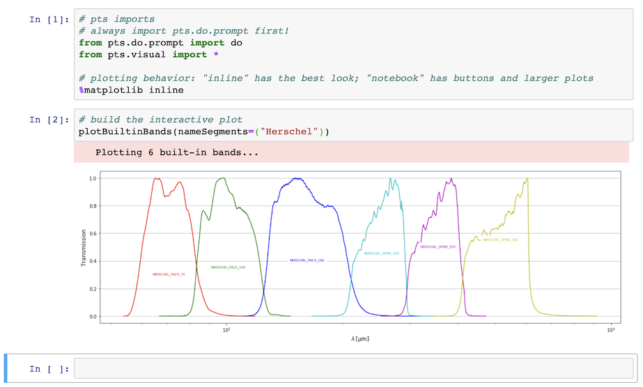
Once properly initialized as described above, any PTS facilities can be imported and used just as they would be in a regular Python script, as discussed in Using PTS in Python programs. The only difference is that plots can be displayed inside the notebook rather than being saved to PDF. Below is a short example.

Furthermore, the pts.do.prompt.do() function (imported by the initialization described above) enables performing a PTS command script as if it were invoked from the command line, as discussed in Using PTS on the command line. For example:

do("list_bands")

will produce:

Starting band/list_bands...
There are 85 built-in bands:
| Band name          | Pivot wavelength
|--------------------|-----------------
| 2MASS_2MASS_J      | 1.2393 micron
| 2MASS_2MASS_H      | 1.6494 micron
| 2MASS_2MASS_KS     | 2.1638 micron
| ALMA_ALMA_10       | 349.89 micron
...