The functionality of PTS is fully available as a set of regular Python packages that can be imported into external Python code. This allows developing custom visualization scripts or even fully automated pipelines without having to start from scratch. This tutorial introduces the basic concepts of how to use PTS from Python by studying a simple example program. For more information on each of the subjects introduced, refer to the PTS Reference documentation.

Getting ready

This tutorial assumes that

you have completed the introductory SKIRT tutorials;
you have reviewed the user guide topics at user level 1;
you have a working knowledge of Python programming;
you have installed SKIRT, PTS, and Python (see Installation Guide).

Note: To allow importing PTS packages into external Python code, the PYTHONPATH environment variable must have been properly defined. This is usually accomplished in the login shell script, and should have been setup during the installation of PTS. For more information, refer to Configuring PTS paths and aliases in the installation guide.

This tutorial offers a ski file for download to serve as a template configuration. Download the file TutorialPythonGalaxy.ski using the link provided in the table below and put it into your local working directory.

Initial SKIRT parameter file	TutorialPythonGalaxy.ski

This ski file describes a panchromatic simulation of a very basic spiral galaxy model including a single instrument and some specific types of probes.

We will introduce the Python program section by section. To work through the tutorial, you can copy each new code section into a regular Python script and run the partially complete program from the start. Alternatively, you can copy the code sections into a Python notebook (see Using PTS in interactive Python notebooks) so that you can run each section separately.

Constructing the program

Importing PTS packages

import logging
import pts.simulation as sm
import pts.utils as ut
import pts.visual as vis
import pts.do
pts.do.initializePTS()

At the start of the script:

Import the PTS packages that will be used; there is a shorthand convention for most packages, as shown above, and as presented in Importing packages in the PTS developer guide.
Initialize the PTS libraries by calling pts.do.initializePTS(); this also configures the standard logging package to include a time stamp in each message.
Usually it is meaningful to import the standard logging package as well, so that your program can emit messages with the same format as the PTS log messages.

Modifying SKIRT parameter files

skifile = sm.SkiFile("TutorialPythonGalaxy.ski")
skifile.setNumPrimaryPackets(1e7)
skifile.saveTo("galaxy.ski")
logging.info("Saved galaxy.ski")

This section of the code reads the ski file you previously downloaded, modifies the number of photon packets being launched in each phase, and saves the updated file under a new name. The pts.simulation.skifile.SkiFile class offers many more functions to obtain information from and/or update the contents of SKIRT configuration files.

Performing SKIRT simulations

logging.info("Executing galaxy.ski")
skirt = sm.Skirt()
simulation = skirt.execute("galaxy.ski", console='brief')

This section of the code employs the pts.simulation.skirt.Skirt class to actually perform the SKIRT simulation. The constructor of this class attempts to locate the SKIRT executable in some default location, which can be overridden using the path argument.

The pts.simulation.skirt.Skirt.execute() function offers various arguments (not used here) to specify the location of the SKIRT input/output files and to control parallelization. The console argument is given the value 'brief' to limit the number of SKIRT log messages written to the console to the most important ones; in any case all messages are still being written to the SKIRT log file as usual.

The execute() function returns an object of type pts.simulation.simulation.Simulation which can be used to access the results of the SKIRT simulation. Note that the actual results reside on disk; the simulation object merely remembers where they are.

simulation = sm.createSimulation(prefix="galaxy")

While invoking SKIRT directly from Python is very useful in automated workflows, there are many situations where this might be impracticle or even impossible (e.g. because running the simulation and analyzing its results is not being done on the same computer). In cases where the simulation has already been performed, the line above creates a simulation object corresponding to its result. The pts.simulation.simulation.createSimulation() function takes an extra argument to specify the location if needed.

Producing built-in visualizations

micron = sm.unit("micron")
vis.plotSeds(simulation, minWavelength=0.1 * micron, maxWavelength=900 * micron,
             decades=4, figSize=(7, 4.5), outFileName="galaxy_sed.pdf")

The built-in visualizations offered from the command line (see Visualizing SKIRT results with PTS) are obviously also available as regular functions, often offering more flexibility through extra arguments. The code section above calls on the pts.visual.plotcurves.plotSeds() function to plot the spectrum observed by the simulation. Note that all quantities in PTS have astropy units attached. In the above example, the wavelengths are specified im micron. See Units and Quantities for more information on the astropy.units package.

The plotSeds() function automatically plots the indvidual components contributing to the total flux because there is only a single instrument in the simulation. Here is the resulting plot:

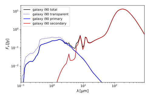
For more information on other visualization options, refer to the reference documentation of the pts.visual package.

Loading FITS files

totalfluxpath = simulation.instruments()[0].outFilePaths(fileType="total.fits")[0]
datacube = sm.loadFits(totalfluxpath)
x,y,wavelengths = sm.getFitsAxes(totalfluxpath)

The first line in this code section obtains the absolute path of the total flux data cube generated by the first instrument in the simulation. In this particular case, we could easily have hardcoded the filename, but the generic method is more instructive. A simulation object can asked for a list of instrument objects, which in turn can be asked for a list of output file paths.

The second line loads the data cube, and the third line loads the three corresponding axes. Note that both the pts.simulation.fits.loadFits() and pts.simulation.fits.getFitsAxes() functions return astropy quantities with units attached. See Units and Quantities for more information on the astropy.units package.

frame = datacube[:,:,20]
wavelength = wavelengths[20]
logging.info("Observed frame has {} by {} pixels".format(*frame.shape))
logging.info("Maximum surface brightness at {:.3f} is {:.3f}".format(wavelength, frame.max()))

This code section arbitrary picks the wavelength with index 20 in the wavelength grid established for the instrument in the ski file and outputs the maximum surface brightness at that wavelength:

Observed frame has 500 by 200 pixels
Maximum surface brightness at 0.643 micron is 1.156 MJy / sr

Note that surface brightness units are automatically included by the astropy units machinery.

Loading text column files

for probe in simulation.probes():
    if "CellProperties" in probe.type():
        filepath = probe.outFilePaths()[0]
        volume, density = sm.loadColumns(filepath, "volume,dust mass density")
        mass = volume*density
    if "Temperature" in probe.type():
        filepath = probe.outFilePaths()[0]
        temperature, = sm.loadColumns(filepath, "indicative temperature")
Tavg = (mass*temperature).sum() / mass.sum()

This code section assumes that the simulation configuration includes a SpatialCellPropertiesProbe and a TemperatureProbe configured with a PerCellForm. The for loop iterates over all probes and selects the appropriate ones.

The pts.simulation.text.loadColumns() function loads specific columns of a text column file, using the structured header information included by SKIRT. The columns to be loaded can be specified as a comma-separated list of header descriptions corresponding to those in the file header. Again, the function returns astropy quantities with appropriate units attached.

In the example above, the cell volumes and dust mass densities written by the SpatialCellPropertiesProbe are combined with the cell temperatures written by the TemperatureProbe to obtain the mass-weighted average dust temperature.

logging.info("Maximum dust temperature is {:.2f}".format(temperature.max()))
logging.info("Maximum cell dust mass is {:.1f}".format(mass.max()))
logging.info("Mass-weighted average dust temperature is {:.2f}".format(Tavg))

This code section simply outputs the calculated results, again automatically including units:

Maximum dust temperature is 21.08 K
Maximum cell dust mass is 9002.1 solMass
Mass-weighted average dust temperature is 17.19 K

The complete program

Here is the complete Python program:

# import and initialize
import logging
import pts.simulation as sm
import pts.utils as ut
import pts.visual as vis
import pts.do
pts.do.initializePTS()
 
# adjust the ski file
skifile = sm.SkiFile("TutorialPythonGalaxy.ski")
skifile.setNumPrimaryPackets(1e7)
skifile.saveTo("galaxy.ski")
logging.info("Saved galaxy.ski")
 
# perform the simulation
logging.info("Executing galaxy.ski")
skirt = sm.Skirt()
simulation = skirt.execute("galaxy.ski", console='brief')
 
# if the simulation has already been performed, use this instead
#simulation = sm.createSimulation(prefix="galaxy")
 
# plot the SED
micron = sm.unit("micron")
vis.plotSeds(simulation, minWavelength=0.1 * micron, maxWavelength=900 * micron,
             decades=4, figSize=(7, 4.5), outFileName="galaxy_sed.pdf")
 
# determine the maximum surface brightness at a certain wavelength
totalfluxpath = simulation.instruments()[0].outFilePaths(fileType="total.fits")[0]
datacube = sm.loadFits(totalfluxpath)
x,y,wavelengths = sm.getFitsAxes(totalfluxpath)
 
frame = datacube[:,:,20]
wavelength = wavelengths[20]
logging.info("Observed frame has {} by {} pixels".format(*frame.shape))
logging.info("Maximum surface brightness at {:.3f} is {:.3f}".format(wavelength, frame.max()))
 
# determine the mass-weighted average dust temperature
for probe in simulation.probes():
    if "CellProperties" in probe.type():
        filepath = probe.outFilePaths()[0]
        volume, density = sm.loadColumns(filepath, "volume,dust mass density")
        mass = volume*density
    if "Temperature" in probe.type():
        filepath = probe.outFilePaths()[0]
        temperature, = sm.loadColumns(filepath, "indicative temperature")
Tavg = (mass*temperature).sum() / mass.sum()
 
logging.info("Maximum dust temperature is {:.2f}".format(temperature.max()))
logging.info("Maximum cell dust mass is {:.1f}".format(mass.max()))
logging.info("Mass-weighted average dust temperature is {:.2f}".format(Tavg))

And here is the complete output generated by the program (replacing some irrelevant material by _):

_ 16:00:30.362   Saved galaxy.ski
_ 16:00:30.363   Executing galaxy.ski
_ 16:00:30.377   Welcome to SKIRT v9.0 (_)
_ 16:00:30.378   Running on _ for _
_ 16:00:30.378   Constructing a simulation from ski file '/_/galaxy.ski'...
_ 16:00:34.989 - Finished setup in 4.6 s.
_ 16:00:35.072 - Finished setup output in 0.1 s.
_ 16:00:55.859 - Finished primary emission in 20.8 s.
_ 16:01:03.953 - Finished secondary emission in 8.1 s.
_ 16:01:03.953 - Finished the run in 28.9 s.
_ 16:01:06.188 - Finished final output in 2.2 s.
_ 16:01:06.188 - Finished simulation galaxy using 16 threads and a single process in 35.8 s.
_ 16:01:06.293   Available memory: 32 GB -- Peak memory usage: 1.08 GB (3.4%)
_ 16:01:07.158   Created /_/galaxy_sed.pdf
_ 16:01:07.275   Observed frame has 800 by 200 pixels
_ 16:01:07.276   Maximum surface brightness at 0.643 micron is 1.156 MJy / sr
_ 16:01:07.355   Maximum dust temperature is 21.08 K
_ 16:01:07.356   Maximum cell dust mass is 9002.1 solMass
_ 16:01:07.357   Mass-weighted average dust temperature is 17.19 K