Lyman-alpha resonant line transfer

This page describes how SKIRT implements Lyman-alpha resonant line transfer. We indicate the assumptions about (or rather restrictions on) the simulated model, summarize the relevant physics, and discuss various aspects of the implementation and the numerical recipes used. To actually enable this capability in a SKIRT simulation, see Configuring for Lyman-alpha resonant line transfer.

Assumptions

Hydrogen is the most abundant element in our Universe and, correspondingly, the Lyman-alpha (Lyα) transition serves as an important observational tool. Because Lyα is a resonance line, and because many astrophysical environments are optically thick at Lyα wavelengths, the related radiative transfer calculations are nontrivial. The implementation of Lyα capabilities in SKIRT is limited to models that conform to the following important assumptions (or rather restrictions):

• The spatial extent of the model is small relative to the distance to the observer (i.e. to the instruments in SKIRT). This allows considering all locations in the model to have the same distance to the observer and it allows using parallel projection.
• The spatial extent of the model is small relative to a cosmological volume and the spatial grid in SKIRT is well-resolved across the model, implying a maximum size of the order of a single galaxy. This allows assuming that the wavelength shifts caused by cosmic expansion within each spatial cell are small relative to the width of the local Lyα cross section profile. (If this would not be the case, a photon packet might inadvertently 'skip' over the cross section profile rather than being scattered.)
• The model is intended to trace the Lyα radiation emerging from the interstellar medium (ISM) that is part of the astrophysical object under study, while ignoring the effects of the circumgalactic and intergalactic medium (CGM/IGM) outside of the object. This avoids the need for providing a larger simulation box and/or including a subgrid recipe for handling the effects of the CGM/IGM.
• The density distribution of neutral hydrogen is defined by the input model and remains fixed during the simulation. In other words, there is no self-consistent calculation of the ionized hydrogen fraction. Instead, the user is responsible for determining this in advance of the radiative transfer simulation.

Within these limitations, the model can be placed at any redshift supported by SKIRT (see Nonzero redshift & CMB dust heating)

Physics

Emission

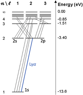
The above diagram illustrates some of the energy levels of atomic hydrogen (labeled with quantum numbers $n,\ell$) and the allowed transitions between them. Whenever the electron ends up on a higher energy level, it cascades down to either the 2s or the 2p state. From the 2p state, the final transition to the ground state produces a Lyα photon, corresponding to a wavelength of ${\lambda }_{\alpha }=1215.67\AA$. From the 2s state, single-photon transitions are forbidden (because they require $\mathrm{\Delta }\ell =\pm 1$), but two-photon transitions allow the electron to decay to the ground state. These transitions are much less probable but still occur frequently enough to justify the assumption that essentially all neutral hydrogen atoms in astrophysical contexts reside in the ground state.

Electrons can end up in a higher energy state in two different ways. The first possibility is by collisions between a free electron and a neutral hydrogen atom, exciting the atom at the expense of kinetic energy of the free electron. The process converts thermal energy of the electrons, and thus of the gas as whole, into radiation. It is therefore also referred to as cooling by producing Lyα radiation. The efficiency of this process depends on the number densities of electrons and neutral hydrogen atoms and on the velocity distribution of the electrons.

The second mechanism is recombination of a free proton and a free electron, which again can leave the electron in any energy state. It is possible to compute the probability that a Lyα photon is produced during the radiative cascade down to the ground-state by summing (and properly weighing) the probabilities for each of the excited states. One usually assumes that astrophysical gases efficiently re-absorb higher order Lyman series and ionizing photons, effectively canceling out these transitions. This on the spot approximation is referred to as Case-B recombination.

For both emission mechanisms, the calculations are complicated and we don't discuss further details here. Instead, we briefly consider the most important astrophysical sites of Lyα production.

Interstellar HII regions are the most prominent sources of Lyα in the Universe. Young stars produce ionizing photons in their atmospheres which are efficiently absorbed in the ISM, and thus create regions of ionized hydrogen. Recombining protons and electrons give rise to Lyα emission (among lines caused by other electronic transitions). For a fixed initial mass function, the Lyα production rate increases towards lower metallicities. Stellar evolution models combined with stellar atmosphere models show that the effective temperature of stars of fixed mass become hotter with decreasing gas metallicity. The increased effective temperature causes a larger fraction of the bolometric luminosity to be emitted as ionizing radiation.

The (usually small) neutral hydrogen fraction in the CGM and IGM can produce spatially extended Lyα emission resulting from cooling (collisions with electrons) or triggered by ionizing radiation from other external sources such as the Universal ultraviolet (UV) background. This internal CGM/IGM emission usually has a low surface brightness, however, and it is often dominated by scattered Lyα radiation that actually originated in remote sources.

Destruction

Photons at or near the Lyα line frequency can be absorbed and scattered by dust grains just like any other photons. Because this process in SKIRT is extensively discussed elsewhere, we don't discuss it here.

Several processes other than dust absorption can destroy Lyα photons, including conversion to another wavelength by certain nearby molecular hydrogen lines, collisional mixing of the atomic hydrogen 2s and 2p energy levels, and photo-ionization of hydrogen atoms that are not in the ground state. These processes are generally less important and we ignore them here.

Scattering

When a Lyα photon is absorbed by a neutral hydrogen atom in the ground state, the atom is excited to the 2p energy level and a new Lyα photon is emitted almost immediately as a result of the subsequent downward transition. This happens fast enough that we can consider the combined process as a scattering event.

The cross section for a single hydrogen atom of the Lyα scattering of a photon can be derived using quantum mechanical considerations, resulting in a sharply peaked profile as a function of the photon wavelength in the atom's rest frame. Because each atom has its own velocity, a photon with a given wavelength in the gas rest frame will appear Doppler shifted to a slightly different wavelength for each atom in the gas. To compute the Lyα absorption cross section for a collection of moving atoms, we must therefore convolve the single-atom cross section with the atom velocity distribution, which in turn depends on the gas temperature.

Assuming a Maxwell-Boltzmann velocity distribution, we define the characteristic thermal velocity $v_{\mathrm{t}\mathrm{h}}$ as

$$v_{\mathrm{t}\mathrm{h}}=\sqrt{\frac{2k_{\mathrm{B}}T}{m_{\mathrm{p}}}}$$

where $k_{\mathrm{B}}$ is the Boltzmann constant, $m_{\mathrm{p}}$ is the proton mass, and $T$ is the temperature of the gas. We then introduce the dimensionless frequency variable $x$, defined as

$$x=\frac{\nu -{\nu }_{\alpha }}{{\nu }_{\alpha }}\frac{c}{v_{\mathrm{t}\mathrm{h}}}=\frac{v_{\mathrm{p}}}{v_{\mathrm{t}\mathrm{h}}}$$

where $\nu =c/\lambda$ is the regular frequency variable, ${\nu }_{\alpha }=c/{\lambda }_{\alpha }$ is the frequency at the Lyα line center, ${\lambda }_{\alpha }$ is the wavelength at the Lyα line center, and $c$ is the speed of light in vacuum. The last equality introduces the velocity shift $v_{\mathrm{p}}$ of the photon frequency relative to the Lyα line center, defined by

$$\frac{v_{\mathrm{p}}}{c}=\frac{\nu -{\nu }_{\alpha }}{{\nu }_{\alpha }}\approx -\frac{\lambda -{\lambda }_{\alpha }}{{\lambda }_{\alpha }}$$

where the approximate equality holds for $v_{\mathrm{p}}\ll c$.

After neglecting some higher order terms, the convolution of the single-atom profile with the Maxwell-Boltzmann velocity distribution yields the following expression for the velocity-weighted Lyα scattering cross section ${\sigma }_{\alpha }(x,T)$ of a hydrogen atom in gas at temperature $T$ as a function of the dimensionless photon frequency $x$:

$${\sigma }_{\alpha }(x,T)={\sigma }_{\alpha ,0}(T)H(a_{\mathrm{v}}(T),x)$$

where the cross section at the line center ${\sigma }_{\alpha ,0}(T)$ is given by

$${\sigma }_{\alpha ,0}(T)=\frac{3{\lambda }_{\alpha }^2{a}_{\mathrm{v}}(T)}{2\sqrt{\pi }},$$

the Voigt parameter $a_{\mathrm{v}}(T)$ is given by

$$a_{\mathrm{v}}(T)=\frac{A_{\alpha }}{4\pi {\nu }_{\alpha }}\frac{c}{v_{\mathrm{t}\mathrm{h}}}$$

with $A_{\alpha }$ the Einstein A-coefficient of the Lyα transition; and the Voigt function $H(a_{\mathrm{v}},x)$ is defined by

$$H(a_{\mathrm{v}},x)=\frac{a_{\mathrm{v}}}{\pi }{\int }_{-\mathrm{\infty }}^{\mathrm{\infty }}\frac{{\mathrm{e}}^{-y^2}\mathrm{d}y}{(y-x{)}^2+a_{\mathrm{v}}^2}$$

which is normalized so that $H(a_{\mathrm{v}},0)\approx 1$ for $a_{\mathrm{v}}\ll 1$.

The Voigt profile is very steep. For typical astrophysical gas temperatures, the Lyα scattering cross section at the line center is more than 10 orders of magnitude larger than the Thomson cross section for scattering by a free electron, indicating the resonant nature of the line. This large cross section leads to line-center optical depths of ${10}^7-{10}^8$ for the typical HI column densities observed in nearby galaxies. However, the Doppler shifts caused by the thermal velocities of the atoms in the gas redistribute the photon's frequency after each scattering event, moving a fraction of the photons into the wings of the Voigt profile, and allowing them to escape more easily from the gas.

Frequency shift due to atom velocity

In most astrophysical conditions, the energy of the Lyα photon before and after scattering is identical in the frame of the interacting atom. This is because the life time of the atom in its 2p state is very short so that it is not perturbed over this short time interval. Because of the random thermal motion of the atom, energy conservation in the atom's frame translates to a change in the energy of the incoming and outgoing photon that depends on the velocity of the atom and the scattering direction. Given the velocity of the atom $\mathbf{v}$, we define the dimensionless atom velocity as $\mathbf{u}=\mathbf{v}/v_{\mathrm{t}\mathrm{h}}$. Denoting the propagation direction and dimensionless frequency of the photon before (after) scattering with ${\mathbf{k}}_{\mathrm{i}\mathrm{n}}$ and $x_{\mathrm{i}\mathrm{n}}$ ( ${\mathbf{k}}_{\mathrm{o}\mathrm{u}\mathrm{t}}$ and $x_{\mathrm{o}\mathrm{u}\mathrm{t}}$), the resulting frequency change can be written as

$$x_{\mathrm{o}\mathrm{u}\mathrm{t}}=x_{\mathrm{i}\mathrm{n}}-\mathbf{u}\cdot {\mathbf{k}}_{\mathrm{i}\mathrm{n}}+\mathbf{u}\cdot {\mathbf{k}}_{\mathrm{o}\mathrm{u}\mathrm{t}}$$

This analysis ignores the energy transferred from the photon to the atom through recoil, an approximation that is justified in regular astrophysical conditions.

Assuming a Maxwell-Boltzmann velocity distribution for the atoms, the two components of the dimensionless atom velocity $\mathbf{u}$ that are orthogonal to the incoming photon direction ${\mathbf{k}}_{\mathrm{i}\mathrm{n}}$ have a Gaussian probability distribution with zero mean and a standard deviation of $1/\sqrt{2}$. The parallel component is more complicated. We denote the dimensionless atom velocity component parallel to the incoming photon direction as $u_{\parallel }$. The probability distribution $P(u_{\parallel }|x_{\mathrm{i}\mathrm{n}})$ for this component is proportional to both the Gaussian atom velocity distribution and the Lyα scattering cross section for a single atom, reflecting the preference for photons to be scattered by atoms to which they appear close to resonance. With the proper normalization this leads to

$$P(u_{\parallel }|x_{\mathrm{i}\mathrm{n}})=\frac{a_{\mathrm{v}}}{\pi H(a_{\mathrm{v}},x_{\mathrm{i}\mathrm{n}})}\frac{{\mathrm{e}}^{-u_{\parallel }^2}}{(u_{\parallel }-x_{\mathrm{i}\mathrm{n}}{)}^2+a_{\mathrm{v}}^2}$$

Scattering phase function

Lyα scattering takes one of two forms: isotropic scattering or dipole scattering; the latter is also called Rayleigh scattering. The corresponding phase functions depend only on the cosine of the scattering angle $\mu ={\mathbf{k}}_{\mathrm{i}\mathrm{n}}\cdot {\mathbf{k}}_{\mathrm{o}\mathrm{u}\mathrm{t}}$. With normalization ${\int }_{-1}^{1}P(\mu )\mathrm{d}\mu =2$ these phase functions can be written, respectively, as

$$P(\mu )=1$$

and

$$P(\mu )=\frac{3}{4}({\mu }^2+1)$$

Quantum mechanical considerations lead to a simple recipe for selecting the appropriate phase function depending on whether the incoming photon frequency is in the core or in the wings of the cross section. The recipe prescribes to treat 1/3 of all core scattering events as dipole, and the remaining 2/3 as isotropic; and to treat all wing scattering events as dipole. For the purpose of this recipe, the scattering event is considered to occur in the core if the incoming dimensionless photon frequency in the rest frame of the interacting atom is smaller than a critical value, $|x|<0.2$.

Overall, a Lyα scattering event affects both the photon direction and frequency in a way that can be described by the redistribution function $R(x_{\mathrm{o}\mathrm{u}\mathrm{t}},x_{\mathrm{i}\mathrm{n}},\mu )$. One can obtain expressions for conditional and marginalized probability distributions derived from this function to enable further analysis and understanding. We just mention two interesting results here. (1) The redistribution of the photon frequency is very similar for isotropic and dipole scattering. (2) Photons that scatter in the wing of the line are pushed back to the line core by an amount of $-1/x_{\mathrm{i}\mathrm{n}}$.

Polarization

A Lyα scattering event also changes the polarization of the involved photon. For the case of isotropic scattering (2/3 of the core events; see previous section), the emitted photon is unpolarized. In other words, the two consecutive electronic state transitions lost all memory of the incoming photon. For the case of dipole scattering (1/3 of the core events and all wing events; see previous section), the polarization state of the photon is adjusted by the scattering event. The transformation of the Stokes vector components is described by the phase matrix, which is also called the Müller matrix (see Polarization by spherical grains).

Assuming that the Stokes vector is properly rotated into the scattering plane, and with the cosine of the scattering angle denoted as $\mu ={\mathbf{k}}_{\mathrm{i}\mathrm{n}}\cdot {\mathbf{k}}_{\mathrm{o}\mathrm{u}\mathrm{t}}$, the phase matrix for Rayleigh (dipole) scattering by a particle with isotropic properties can be written as

$${\mathbf{M}}_{\mathrm{d}\mathrm{i}\mathrm{p}}(\mu )\propto \left(\begin{array}{cccc}{\mu }^2+1& {\mu }^2-1& 0& 0\\ {\mu }^2-1& {\mu }^2+1& 0& 0\\ 0& 0& 2\mu & 0\\ 0& 0& 0& 2\mu \end{array}\right)$$

where the proportionality factor is irrelevant. Note that this is the same phase matrix as the one for Thomson scattering of photons by free electrons.

Hubble flow

Cosmological simulations usually output peculiar velocities, not physical ones. That is, the velocity field imported from the simulation snapshot is the velocity field excluding the effects of cosmological expansion, called the Hubble flow. For example, to determine whether a set of particles/cells form a bound system, one needs to take into account that the snapshot velocity represents just the deviation of the physical velocities from the Hubble flow. Given the extremely peaked form of the Lyα scattering cross section, the wavelength shifts resulting from the Hubble flow may be significant in this context.

Specifically, the Hubble flow velocity shift $\mathrm{\Delta }{v}_{\mathrm{h}}$ corresponding to a photon packet path length $\mathrm{\Delta }s$ is obtained from the Hubble law

$$\mathrm{\Delta }{v}_{\mathrm{h}}=H(z)\mathrm{\Delta }s$$

where, for a flat cosmology (see Nonzero redshift & CMB dust heating), the Hubble parameter $H(z)$ at redshift $z$ is given by

$$H(z)=H_0\sqrt{{\mathrm{\Omega }}_{\mathrm{m}}(1+z{)}^3+(1-{\mathrm{\Omega }}_{\mathrm{m}})}.$$

As long as $\mathrm{\Delta }{v}_{\mathrm{h}}\ll c$, the photon packet wavelength shift corresponding to $\mathrm{\Delta }{v}_{\mathrm{h}}$ can be obtained as usual.

The Hubble flow wavelength shift must evaluated and applied to a photon packet after each cell crossing because the Lyα cross section in subsequent cells depends on the adjusted wavelength. This mechanism assumes that the wavelength shift within each spatial cell are small relative to the width of the local Lyα cross section profile. If this would not be the case, a photon packet might inadvertently 'wavelength-skip' over the cross section profile rather than being scattered.

Numerical recipes

The Voigt function

The Voigt function defined in section Scattering can be evaluated numerically using one of several published approximations. Similarly, the probability distribution in section Frequency shift due to atom velocity can be sampled using one of several published methods. The mechanisms employed by SKIRT are described for the functions in the VoigtProfile namespace.

Photon cycle

The Lyα-with-dust photon cycle generally proceeds in the same way as the dust-only photon cycle. The main, straightforward differences are outlined in this section. Further differences related to acceleration and efficiency are discussed in later sections.

The Lyα optical depth in a spatial cell is calculated as ${\tau }_{\alpha }={\sigma }_{\alpha }{n}_{\mathrm{H}\mathrm{I}}\mathrm{\Delta }s$ where ${\sigma }_{\alpha }(x,T)$ is the Lyα cross section, $x$ is the dimensionless photon packet frequency in the rest frame of the cell, $T$ is the temperature of the gas in the cell, $n_{\mathrm{H}\mathrm{I}}$ is the total neutral hydrogen number density in the cell, and $\mathrm{\Delta }s$ is the length of the path segment crossing the cell. The result is added to the optical depth of the dust components in the cell.

When the spatial cell containing the location for a scattering event has been determined, the interacting medium component is selected at random from the discrete distribution formed by the local scattering opacities $k_h$ for each component $h$, using the perceived photon packet wavelength in the medium's rest frame. For Lyα, the scattering opacity equals the total opacity $k_{\alpha }={\sigma }_{\alpha }{n}_{\mathrm{H}\mathrm{I}}$ because there is no absorption. In case a Lyα component is selected as the interacting medium, the scattering operation proceeds as described for the LyaUtils::sampleAtomVelocity() function.

For photon packets peeled off a scattering event, the contribution of each medium component $h$ is weighted by the local scattering opacities $k_h$ calculated as described above for the regular scattering event. The peel-off photon packet direction is now determined by the position of the instrument rather than sampled from the phase function. However, the phase function is still required to calculate the bias factor to be applied to the luminosity of the photon packet. All peel-offs for a given scattering event must use the same atom velocity and the same phase function as the actual scattering event. This keeps the peel-offs consistent with the scattering event, and it avoids expensive calculations to sample a new atom velocity for each peel-off. The relevant information is cached in the photon packet and reused when applicable.

Core-skipping acceleration

In a high-optical-depth medium, the number of scatterings for photon packets near the Lyα line is so high, and the corresponding free path lengths so short, that the Monte Carlo photon cycle becomes prohibitively slow. The core-skipping acceleration mechanism used by many authors forces the wavelength of photon packets from the core of the Lyα line into the wings of the line, reducing the scattering cross section and allowing the photon packet to escape. This is acceptable because for these consecutive core scatterings the following assumptions are justified: (a) the mean free path length between the scattering locations is sufficiently small that the resulting extinction by dust is negligible, and (b) the effects of the phase function on the scattering direction and polarization state are essentially randomized by the large number of scattering events.

The acceleration scheme employs a critical frequency $x_{\mathrm{c}\mathrm{r}\mathrm{i}\mathrm{t}}$ that indicates the transition from core to wing. Photons in the wings ( $|x|>x_{\mathrm{c}\mathrm{r}\mathrm{i}\mathrm{t}})$) receive no special treatment. Photons in the core ( $|x|<x_{\mathrm{c}\mathrm{r}\mathrm{i}\mathrm{t}}$) are accelerated as follows. Ordinarily, the physical mechanism that puts a Lyα photon from the core into the wing of the line profile is an encounter with a fast moving atom. We can force the scattering atom to have a large velocity when generating its velocity components.

A simple way to do this is by forcing the velocity component of the atom perpendicular to the incoming photon packet, ${\mathbf{v}}_{\mathrm{\perp }}$, to be large. We know from section Frequency shift due to atom velocity that the magnitude of this component, $v_{\mathrm{\perp }}=||{\mathbf{v}}_{\mathrm{\perp }}\mathbf{|}\mathbf{|}$, follows a 2D Gaussian distribution. In dimensionless units $u_{\mathrm{\perp }}=v_{\mathrm{\perp }}/v_{\mathrm{t}\mathrm{h}}$, this can be written as $g(u_{\mathrm{\perp }})\propto u_{\mathrm{\perp }}\exp (-u_{\mathrm{\perp }}^2)$. We can force $u_{\mathrm{\perp }}$ to be large by drawing it instead from a truncated distribution,

$$P(u_{\mathrm{\perp }})\propto \{\begin{array}{ll}0& |u_{\mathrm{\perp }}|<x_{\mathrm{c}\mathrm{r}\mathrm{i}\mathrm{t}}\\ u_{\mathrm{\perp }}{\mathrm{e}}^{-u_{\mathrm{\perp }}^2}& |u_{\mathrm{\perp }}|>x_{\mathrm{c}\mathrm{r}\mathrm{i}\mathrm{t}}\end{array}$$

where the proportionality factor is chosen so that the distribution is properly normalized, and $x_{\mathrm{c}\mathrm{r}\mathrm{i}\mathrm{t}}$ determines how far into the wing we force the Lyα photon packets. This parameter therefore sets by how much Lyα transfer is accelerated. The two components of $u_{\mathrm{\perp }}$ can be sampled using

$$\begin{array}{rl}{u}_{\mathrm{\perp },a}& =\sqrt{x_{\mathrm{c}\mathrm{r}\mathrm{i}\mathrm{t}}^2-\ln {\mathcal{X}}_1}\cos (2\pi {\mathcal{X}}_2)\\ u_{\mathrm{\perp },b}& =\sqrt{x_{\mathrm{c}\mathrm{r}\mathrm{i}\mathrm{t}}^2-\ln {\mathcal{X}}_1}\sin (2\pi {\mathcal{X}}_2)\end{array}$$

where ${\mathcal{X}}_1$ and ${\mathcal{X}}_2$ are uniform deviates.

Acceleration schemes in SKIRT

SKIRT implements three variations of the core-skipping acceleration scheme:

• None: no acceleration is performed, corresponding to $x_{\mathrm{c}\mathrm{r}\mathrm{i}\mathrm{t}}=0$. This can be useful for models with low optical depths, or to produce reference results for models with medium optical depths. For models with high optical depths, the run times will be prohibitively long.
• Constant: acceleration with a constant critical value given by $x_{\mathrm{c}\mathrm{r}\mathrm{i}\mathrm{t}}=3s$, where $s$ is the acceleration strength configured by the user. This option can be useful when the optical depth is fairly constant throughout the model, as is the case with many benchmark models.
• Variable: acceleration with a variable critical value that depends on the local gas temperature and density. Specifically, the critical value is determined as

  $$x_{\mathrm{c}\mathrm{r}\mathrm{i}\mathrm{t}}=s{\left(\frac{n_{\mathrm{H}}}{T}\right)}^{1/6},$$

  where $s$ is the acceleration strength configured by the user and $n_{\mathrm{H}}$ is the neutral hydrogen number density (in ${\mathrm{m}}^{-3}$) and $T$ the gas temperature (in K) in the spatial cell hosting the scattering event. The rationale behind this formula is discussed below. This variable mechanism is applicable for most models, and is preferred for models with a broad dynamic range in optical depths.

For both the constant and variable schemes, the user can configure the acceleration strength $s$, with a default value of unity. Larger values will decrease run time and accuracy; smaller values will increase run time and accuracy.

Rationale for the variable scheme

The approximate analytical solutions for the Lyα spectrum emerging from a static slab or sphere (Neufeld 1990, Dijkstra et al. 2006) depend on the product $a{\tau }_0$, where $a$ is the Voigt parameter and ${\tau }_0$ is the optical depth at the Lyα line center. Inspired by this result, many authors proposed acceleration schemes where $x_{\mathrm{c}\mathrm{r}\mathrm{i}\mathrm{t}}$ is determined as a function of this product. For example, Smith et al. 2015 (MNRAS, 449, 4336-4362) used a critical value proportional to $(a{\tau }_0{)}^{1/3}$.

However, calculating the optical depth requires selecting a path length. This has forced these schemes to depend on either a local scale (such as the size of the current spatial cell) or a global scale (such as the domain size). Both options seem undesirable, as they lead to a dependency on non-physical parameters (the resolution of the discretization or the portion of the physical world included in the model). Interestingly, Smith et al. 2015 (MNRAS, 449, 4336-4362) noted that one could use the Jeans length as a physically motivated length scale. Expressing the Jeans length as well as the other quantities in $(a{\tau }_0{)}^{1/3}$ as a function of the local gas properties leads to $x_{\mathrm{c}\mathrm{r}\mathrm{i}\mathrm{t}}\propto (n_{\mathrm{H}}/T{)}^{1/6}$. With the gas properties expressed in SI units, experiments with benchmark models show that a proportionality factor of order unity is appropriate.

Path calculation and forced scattering

SKIRT employs forced scattering to keep photon packets from escaping the simulation domain. This requires the complete photon packet path to be calculated from each interaction point (emission or scattering) to the outer spatial domain boundary, including grid traversal and optical depth along the path segment crossing each cell. The resulting information is used to calculate the escape fraction and to determine the location of the next scattering event. The technique substantially accelerates the photon cycle for models with low or limited optical depths, where photon packets would easily escape.

However, photon packets near the Lyα line routinely encounter extremely high optical depths. Even with the acceleration schemes discussed in the previous section, Lyα photon packets often undergo a large number of scattering events; it is not unusual for a packet to scatter many thousands of times. Many of these scattering events are located in the same or in an immediately neighboring spatial cell. Still, the forced scattering implementation calculates the complete path to the outer domain boundary after each scattering event. This causes a tremendous amount of overhead, while in fact there is no need to apply the forced scattering technique in high-optical depth environments because the photon packets rarely escape anyway. It is thus highly recommended to disable forced scattering in Lyα simulations.