 |
The SKIRT project
advanced radiative transfer for astrophysics
|
|
The SKIRT project
advanced radiative transfer for astrophysics
|
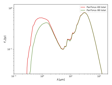
In this tutorial you will use SKIRT to produce the spectral energy distribution (see illustration above) and a full data cube for a dust torus surrounding a central stellar source. You will create a ski file containing the appropriate simulation parameters, perform the simulation, and review and interpret the simulation results.
This tutorial assumes that you have completed the introductory SKIRT tutorial Monochromatic simulation of a dusty disk galaxy, or that you have otherwise acquired the working knowledge introduced there. At the very least, before starting this tutorial, you should have installed the SKIRT code, and preferably also PTS and a FITS file viewer such as DS9 (see Installation Guide).
In a terminal window, with an appropriate current directory, start SKIRT without any command line arguments. SKIRT responds with a welcome message and starts an interactive session in the terminal window, during which it will prompt you for all the information describing a particular simulation:
   Welcome to SKIRT v___
   Running on ___ for ___
   Interactively constructing a simulation...
 ? Enter the name of the ski file to be created: PanTorus
The first question is for the filename of the ski file. For this tutorial, enter "PanTorus".
In this and subsequent tutorials, we skip the questions for which there is only one possible answer. The answers to these questions are provided without prompting the user, and listing them here would bring no added value.
   Possible choices for the user experience level:
      1. Basic: for beginning users (hides many options)
      2. Regular: for regular users (hides esoteric options)
      3. Expert: for expert users (hides no options)
 ? Enter one of these numbers [1,3] (2): 1
As discussed in the previous tutorial (see Experience level), the Q&A session can be tailored to the experience level of the user. Because the current tutorial is intended for beginning users, select Basic level.
   Possible choices for the units system:
      1. SI units
      2. Stellar units (length in AU, distance in pc)
      3. Extragalactic units (length in pc, distance in Mpc)
 ? Enter one of these numbers [1,3] (3): 2
   Possible choices for the output style for wavelengths:
      1. As photon wavelength: λ
      2. As photon frequency: ν
      3. As photon energy: E
 ? Enter one of these numbers [1,3] (1):
   Possible choices for the output style for flux density and surface brightness:
      1. Neutral: λ F_λ = ν F_ν
      2. Per unit of wavelength: F_λ
      3. Per unit of frequency: F_ν
      4. Counts per unit of energy: F_E
  ? Enter one of these numbers [1,4] (3):
As discussed in the previous tutorial (see Units), SKIRT offers several output unit options. For the current tutorial, you will be setting up a dust torus surrounding a stellar source, so it is most convenient to use stellar units with sizes expressed in astronomical units. Select the wavelength output style for the spectral variable and the per unit of frequency style for fluxes (expressing integrated flux density in Jy and surface brightness in MJy/sr).
   Possible choices for the overall simulation mode:
      1. No medium - oligochromatic regime (a few discrete wavelengths)
      2. Extinction only - oligochromatic regime (a few discrete wavelengths)
      3. No medium (primary sources only)
      4. Extinction only (no secondary emission)
      5. Extinction only with Lyman-alpha line transfer
      6. With secondary emission from dust
      7. With secondary emission from gas
      8. With secondary emission from dust and gas
 ? Enter one of these numbers [1,8] (4): 6
As discussed in the previous tutorial (see Simulation mode), the answer to this question determines the wavelength regime of the simulation (oligochromatic or panchromatic) and sets the overall scheme for handling media in the simulation.
For this tutorial, you want SKIRT to produce a full radiation spectrum spanning ultraviolet to submillimeter wavelengths and including the effects of both primary and secondary emission (a stellar source and thermal dust emission). In other words, you need the panchromatic wavelength regime "with secondary emission from dust".
? Enter the default number of photon packets launched per simulation segment [0,1e19] (1e6): 1e7
Because the simulation in this tutorial covers a broad wavelength range, the number of photon packets must be higher than the default value to obtain an acceptable signal to noise ratio. Keep in mind though that the run time of a SKIRT simulation is roughly proportional to the number of photon packets being launched. To limit the run time for this tutorial, set the number of photon packets to \(10^7\). This number is sufficient to produce a reasonable SED for the simple 2D tutorial model, but the frames in the data cube will be quite noisy.
 ? Enter the shortest wavelength of photon packets launched from primary sources [1e-6 micron,1e6 micron] (0.09 micron):
 ? Enter the longest wavelength of photon packets launched from primary sources [1e-6 micron,1e6 micron] (100 micron):
For a panchromatic simulation, the source system requests the limits of the wavelength range to be considered for primary sources. For this tutorial, simply accept the suggested default values, yielding a range of \(0.09~\mu{\text{m}} <= \lambda <= 100~\mu{\text{m}}\).
   Possible choices for item #1 in the primary sources list:
      1. A primary point source
      2. A primary source with a built-in geometry
      3. A primary source imported from smoothed particle data
         ...
 ? Enter one of these numbers or zero to terminate the list [0,6] (2): 1
 ? Enter the position of the point source, x component ]-∞ AU,∞ AU[ (0 AU):
 ? Enter the position of the point source, y component ]-∞ AU,∞ AU[ (0 AU):
 ? Enter the position of the point source, z component ]-∞ AU,∞ AU[ (0 AU):
The primary source for this tutorial is modeled by a point source at the origin. Select "a primary point source" from the offered list of options, and leave its position coordinates at the default value of zero.
   Possible choices for the spectral energy distribution for the source:
      1. A black-body spectral energy distribution
      2. The spectral energy distribution of the Sun
         ...
 ? Enter one of these numbers [1,9] (1): 2
   Possible choices for the type of luminosity normalization for the source:
      1. Source normalization through the integrated luminosity for a given wavelength range
      2. Source normalization through the specific luminosity at a given wavelength
      3. Source normalization through the specific luminosity for a given wavelength band
 ? Enter one of these numbers [1,3] (1): 1
   Possible choices for the wavelength range for which to provide the integrated luminosity:
      1. The wavelength range of the primary sources
      2. All wavelengths (i.e. over the full SED)
      3. A custom wavelength range specified here
 ? Enter one of these numbers [1,3] (1): 2
 ? Enter the integrated luminosity for the given wavelength range ]0 Lsun,∞ Lsun[: 1
As with any other source, you need to provide its emission spectrum and luminosity. SKIRT offers several built-in options for this purpose. For this tutorial, specify the solar emission spectrum normalized to the bolometric luminosity of the Sun. When asked for a second stellar component, enter zero to terminate the list.
   Possible choices for the wavelength grid for storing the radiation field:
      1. A logarithmic wavelength grid
      2. A nested logarithmic wavelength grid
      3. A linear wavelength grid
         ...
 ? Enter one of these numbers [1,7] (1): 1
 ? Enter the shortest wavelength [1e-6 micron,1e6 micron]: 0.09
 ? Enter the longest wavelength [1e-6 micron,1e6 micron]: 100
 ? Enter the number of wavelength grid points [2,2000000000] (25):
Primary sources assign randomly sampled wavelengths to the launched photon packets. These wavelengths can have any floating point value in the primary source range configured for the simulation (here \(0.09~\mu{\text{m}} <= \lambda <= 100~\mu{\text{m}}\)). However, it is impossible to use a similar "infinite" resolution when recording wavelength dependent information on the radiation field in each spatial cell. By necessity, this information must be stored in a finite number of wavelength bins. Because there may be many spatial cells in the simulation, the number of wavelength bins used for storing the radiation field has a substantial effect on the memory consumption of the simulation.
SKIRT offers several types of wavelength grids that can be used for discretizing a wavelength range. For example:
For storing the radiation field in this tutorial simulation, configure a logarithmic wavelength grid with a range that matches the primary source range ( \(0.09~\mu{\text{m}} <= \lambda <= 100~\mu{\text{m}}\)) and has the default number of 25 bins.
   Possible choices for the wavelength grid for calculating the dust emission spectrum:
      1. A logarithmic wavelength grid
      2. A nested logarithmic wavelength grid
      3. A linear wavelength grid
         ...
 ? Enter one of these numbers [1,7] (1): 1
 ? Enter the shortest wavelength [1e-6 micron,1e6 micron]: 1
 ? Enter the longest wavelength [1e-6 micron,1e6 micron]: 1000
 ? Enter the number of wavelength grid points [2,2000000000] (25): 100
Similarly, the thermal emission spectrum for the dust in each spatial cell can only be calculated at a finite number of wavelength grid points. This calculation happens on the fly, i.e. the spectrum does not need to be stored for all spatial cells at the same time. As a result, the impact of the number of wavelength grid points on memory consumption is limited, but there will still be an impact on performance.
For calculating the dust emission spectrum in this tutorial simulation, configure a logarithmic wavelength grid with a range of \(1~\mu{\text{m}} <= \lambda <= 1000~\mu{\text{m}}\) and with 100 wavelength grid points.
   Possible choices for item #1 in the transfer media list:
      1. A transfer medium with a built-in geometry
      2. A transfer medium imported from smoothed particle data
         ...
 ? Enter one of these numbers [1,5] (1):
The medium system in this tutorial simulation contains just a single built-in component describing a torus. So you need to select the "built-in geometry" medium component type.
   Possible choices for the geometry of the spatial density distribution for the medium:
      1. A Plummer geometry
         ...
      9. A torus geometry
         ...
 ? Enter one of these numbers [1,21] (1): 9
 ? Enter the radial powerlaw exponent p of the torus [0,∞[: 0
 ? Enter the polar index q of the torus [0,∞[: 0
 ? Enter the half opening angle of the torus [0 deg,90 deg]: 10
 ? Enter the minimum radius of the torus ]0 AU,∞ AU[: 0.5
 ? Enter the maximum radius of the torus ]0 AU,∞ AU[: 40
For this tutorial, select a torus geometry with a uniform density distribution (hence the zero values for the power-law exponent and the polar index), a half opening angle of 10 degrees and a radius range from 0.5 to 40 AU. A uniform dust density distribution is not very realistic, but it facilitates interpreting the results of this tutorial simulation.
   Possible choices for the material type and properties throughout the medium:
      1. A typical interstellar dust mix (mean properties)
      2. A THEMIS (Jones et al. 2017) dust mix
      3. A Draine and Li (2007) dust mix
      4. A Zubko et al. (2004) dust mix
         ...
 ? Enter one of these numbers [1,10] (1): 4
 ? Enter the number of silicate grain size bins [1,2000000000] (5):
 ? Enter the number of graphite grain size bins [1,2000000000] (5):
 ? Enter the number of neutral and ionized PAH size bins (each) [1,2000000000] (5):
In addition to the spatial distribution of the dust, you need to provide its optical and calorimetric properties. SKIRT offers a wide range of options to define material properties. On the most basic level, SKIRT includes built-in dust mixes that offer "mean" properties only. With these mean properties SKIRT can produce an exact solution for dust extinction effects, but not for thermal dust emission. A more accurate calculation of the dust emission spectrum requires specification of the material properties and grain size distribution for each type of dust material seperately. SKIRT includes some "turn-key" dust mixes that provide this level of detail and require very little extra configuration. On the other hand, it is also possible to specify a custom dust mix with fully configurable grain compositions and size distributions.
For this tutorial, select the "Zubko et al. 2004" turn-key dust mix, which describes the properties for a specific dust model including graphite, silicate and PAH dust grains. Leave the number of size bins for each grain type to the default value of 5.
   Possible choices for the type of normalization for the amount of material:
      1. Normalization by defining the total mass
      2. Normalization by defining the total number of entities
      3. Normalization by defining the optical depth along a coordinate axis
      4. Normalization by defining the mass column density along a coordinate axis
      5. Normalization by defining the number column density along a coordinate axis
 ? Enter one of these numbers [1,5] (3): 3
   Possible choices for the axis along which to specify the normalization:
      1. The X axis of the model coordinate sytem
      2. The Y axis of the model coordinate sytem
      3. The Z axis of the model coordinate sytem
 ? Enter one of these numbers [1,3] (3): 1
 ? Enter the wavelength at which to specify the optical depth [0.0001 micron,1e6 micron]: 0.55
 ? Enter the optical depth along this axis at this wavelength ]0,∞[: 2
You now need to define the amount of dust in the medium component through some normalization. For this tutorial, specify an edge-on optical depth for the torus of \(\tau^\mathrm{e}_V=1\) at a central V band wavelength of \(\lambda=0.55~\mu{\text{m}}\). Note that the edge-on optical depth is defined by integrating along the X-axis from the center of the coordinate axis to infinity, while the normalization in SKIRT assumes integration over the complete X-axis. Because the torus is axisymmetric, the optical depth along the complete X-axis is twice the optical depth along half the X-axis.
Finally, when asked for the second medium component, terminate the list by entering zero.
   Possible choices for the spatial grid:
      1. An axisymmetric spatial grid in cylindrical coordinates
      2. A Cartesian spatial grid
      3. A tree-based spatial grid
 ? Enter one of these numbers [1,3] (1):
 ? Enter the cylindrical radius of the grid ]0 AU,∞ AU[: 40
 ? Enter the start point of the cylinder in the Z direction ]-∞ AU,∞ AU[: -10
 ? Enter the end point of the cylinder in the Z direction ]-∞ AU,∞ AU[: 10
   Possible choices for the bin distribution in the radial direction:
      1. A linear mesh
      2. A power-law mesh
      3. A symmetric power-law mesh
      4. A logarithmic mesh
 ? Enter one of these numbers [1,4] (1): 2
 ? Enter the number of bins in the mesh [1,100000] (100): 100
 ? Enter the bin width ratio between the last and the first bin ]0,∞[ (1): 20
   Possible choices for the bin distribution in the Z direction:
      1. A linear mesh
      2. A power-law mesh
      3. A symmetric power-law mesh
 ? Enter one of these numbers [1,3] (1): 3
 ? Enter the number of bins in the mesh [1,100000] (100): 100
 ? Enter the bin width ratio between the outermost and the innermost bins ]0,∞[ (1): 20
The spatial grid for this tutorial simulation can be two-dimensional, and needs more resolution in the center of the model. Select a 2D axisymmetric dust grid in cylindrical coordinates with a power-law mesh in the radial direction and a symmetric power-law mesh in the vertical direction. Specify a grid radius of 40 AU and a grid height of 20 AU centered on the origin, neatly enclosing the dust torus in the model. Specify 100 cells in each direction, and specify a ratio of the width of the outermost to the innermost bin of 20 in both directions.
   Possible choices for the default instrument wavelength grid:
      1. A logarithmic wavelength grid
      2. A nested logarithmic wavelength grid
         ...
 ? Enter one of these numbers [1,8] (1): 1
 ? Enter the shortest wavelength [1e-6 micron,1e6 micron]: 0.09
 ? Enter the longest wavelength [1e-6 micron,1e6 micron]: 1000
 ? Enter the number of wavelength grid points [2,2000000000] (25): 200
Similar to the situation with recording the radiation field, instruments need to detect and store wavelength dependent flux contributions in a finite number of wavelength bins. The default instrument wavelength grid defines these bins for all instruments and for all probes that output wavelength dependent information. (When running the Q&A with a user experience level higher than Basic, it is possible to assign a different wavelength grid to each instrument or probe.)
For this tutorial, configure a logarithmic wavelength grid with a range of \(0.09~\mu{\text{m}} <= \lambda <= 1000~\mu{\text{m}}\), including both the primary and secondary source wavelength ranges, and with 200 wavelength grid points.
   Possible choices for item #1 in the instruments list:
      1. A distant instrument that outputs the spatially integrated flux density as an SED
      2. A distant instrument that outputs the surface brightness in every pixel as a data cube
      3. A distant instrument that outputs both the flux density (SED) and surface brightness (data cube)
 ? Enter one of these numbers or zero to terminate the list [0,3] (1): 3
 ? Enter the name for this instrument: i00
 ? Enter the distance to the system ]0 pc,∞ pc[: 100
 ? Enter the inclination angle θ of the detector [0 deg,180 deg] (0 deg): 0
 ? Enter the total field of view in the horizontal direction ]0 AU,∞ AU[: 80
 ? Enter the number of pixels in the horizontal direction [1,10000] (250): 800
 ? Enter the total field of view in the vertical direction ]0 AU,∞ AU[: 80
 ? Enter the number of pixels in the vertical direction [1,10000] (250): 800
 ? Do you want to record flux components separately? [yes/no] (no):
   Possible choices for item #2 in the instruments list:
      1. A distant instrument that outputs the spatially integrated flux density as an SED
      2. A distant instrument that outputs the surface brightness in every pixel as a data cube
      3. A distant instrument that outputs both the flux density (SED) and surface brightness (data cube)
 ? Enter one of these numbers or zero to terminate the list [0,3] (1): 3
 ? Enter the name for this instrument: i90
 ? Enter the distance to the system ]0 pc,∞ pc[: 100
 ? Enter the inclination angle θ of the detector [0 deg,180 deg] (0 deg): 90
   ... [remaining questions: same answers as for first instrument]
   ...
For this tutorial, the intention is to create both an SED and an integral field data cube for each line of sight under study, i.e. a face-on view and an edge-on view. Therefore, you need to include two instruments of the default type "outputs both the flux density (SED) and surface brightness (data cube)". For the first instrument, specify an inclination of 0 degrees and a corresponding name, such as "i00" or "faceon". For the second instrument, specify an inclination of 90 degrees and a name such as "i90" or "edgeon". For both instruments, specify a distance of 100 pc, and a field of view of 80 AU and 800 pixels in both directions. Configure the instruments not to record flux components in addition to the total flux.
When asked for a third instrument, enter zero to terminate the list.
   Possible choices for item #1 in the probes list:
      1. Convergence: information on the spatial grid
      2. Convergence: cuts of the medium density along the coordinate planes
      3. Source: luminosities of primary sources
      4. Internal spatial grid: density of the medium
      5. Internal spatial grid: opacity of the medium
      6. Internal spatial grid: indicative temperature of the medium
      7. Properties: basic info for each spatial cell
      8. Properties: data files for plotting the structure of the grid
      9. Properties: aggregate optical material properties for each medium
 ? Enter one of these numbers or zero to terminate the list [0,9] (1): 1
 ? Enter the name for this probe: cnv

   Possible choices for item #2 in the probes list:
         ...
      2. Convergence: cuts of the medium density along the coordinate planes
         ...
 ? Enter one of these numbers or zero to terminate the list [0,9] (1): 2
 ? Enter the name for this probe: dns

   Possible choices for item #3 in the probes list:
         ...
      6. Internal spatial grid: indicative temperature of the medium
         ...
 ? Enter one of these numbers or zero to terminate the list [0,9] (1): 6
 ? Enter the name for this probe: tmp
   Possible choices for the form describing how this quantity should be probed:
      1. Default planar cuts along the coordinate planes
      2. A text column file with values for each spatial cell
 ? Enter one of these numbers [1,2] (1): 1

   Possible choices for item #4 in the probes list:
         ...
 ? Enter one of these numbers or zero to terminate the list [0,9] (1): 0
Configure the following probes, in arbitrary order, and specify their names as follows.
| Probe type | Probe name |
|---|---|
| Convergence: information on the spatial grid | cnv |
| Convergence: cuts of the medium density along the coordinate planes | dns |
| Internal spatial grid: indicative temperature of the medium | tmp |
For the temperature probe, you can choose the "form" in which the quantity should be probed. This is so because various types of output can be produced for a given quantity (in this case the temperature). In Basic mode, there are just two options: FITS files showing a planar cut along each coordinate plane, or a text file listing the temperature for every cell in the spatial grid. In Regular mode, additional options become available, including for example parallel projection along a specified line of sight. For this tutorial, select the option to produce planar cuts along the coordinate planes.
Finally, when asked for the subsequent probe, enter zero to terminate the list.
Once the ski file has been created, you can run the simulation by entering the following command with the same current directory:
$ skirt PanTorus
The SKIRT progress log reflects the various stages of the similation. This panchromatic simulation run includes a secondary emission phase in addition to the primary emission phase. During the primary emission phase, SKIRT tracks the strength of radiation field in each spatial cell at each wavelength in the configured radiation field wavelength grid. During the secondary emission phase, SKIRT uses this information to calculate the secondary dust emission spectrum in each spatial cell.
 ! SunSED available spectrum does not fully cover the configured source wavelength range
 !   Configured: 0.09 micron - 100 micron
 !   Available: 0.0915 micron - 160 micron
   ...
 ! ZubkoDustMix dust properties are not available for full simulation wavelength range
 !   Required: 0.0769 micron - 2.02e+03 micron
 !   Available: 0.001 micron - 1e+03 micron
During setup, SKIRT issues two warning messages. The first one states that the solar spectrum is not available for the complete source wavelength range ( \(0.09~\mu{\text{m}} <= \lambda <= 1000~\mu{\text{m}}\)) requested in the parameter file. Upon closer inspection, the missing range is very small so this will have no significant effect on the simulation results. The second warning indicates that the optical properties for the Zubko et al. 2004 dust model are not available for wavelengths longer than \(1000~\mu{\text{m}}\). Even if the parameter file for this tutorial does not specify any wavelengths beyond \(1000~\mu{\text{m}}\), SKIRT uses wavelengths up to slightly over \(2000~\mu{\text{m}}\) to calculate the dust temperature based on the radiation field, causing this warning. However, the effect on the simulation results will again be negligible. Hence, in this case, you can safely ignore these warnings.
Most of the output files for this tutorial are similar to those already described for the previous tutorial (see Output files). This section describes the output file types that are new to this tutorial.
The instruments used in this tutorial each produce two files:
PanTorus_iNN_total.fits is a FITS file containing the data cube with the total surface brightness for each pixel as detected by the instrument. The data cube has a frame for each wavelength in the instrument's wavelength grid.PanTorus_iNN_sed.dat is a column text data file representing the spectral energy distribution of the photon packets detected by the instrument; there are two columns (wavelength, flux) that can easily be plotted.There are some additional files produced by the temperature probe (named "tmp" in the table above):
PanTorus_tmp_dust_T_xy.fits & PanTorus_tmp_dust_T_xz.fits are FITS data files containing a 1024 x 1024 pixel map of the indicative dust temperature in a coordinate plane, across the total extent of the spatial grid.For dust media, the output of the temperature probe is meaningful only for panchromatic simulations that track the radiation field over a sufficiently wide wavelength range to properly calculate the thermal state of the dust grains. Furthermore, the indicative dust temperature calculated by this probe does not correspond to a physical temperature. The dust grain population of a typical dust mix, when embedded in a particular radiation field, shows a temperature distribution rather than a single temperature. To calculate the indicative dust temperature for a given spatial cell, SKIRT uses a straightforward averaging mechanism. However, there are several methods to obtain such a representative temperature, and in general each method yields a different value.
As always it is a good idea to open the file PanTorus_cnv_convergence.dat in a text editor and check the dust grid convergence metrics. The expected values should be within a few percent of the actual values. It is also instructive to compare the theoretical and gridded dust density cuts (e.g. PanTorus_dns_dust_t_xz.fits and PanTorus_dns_dust_g_xz.fits) in an interactive FITS viewer or by plotting them using the following PTS command:
pts plot_convergence . --prefix=PanTorus --dex 2
Note, for example, the grid effects and the varying cell sizes at the edges of the torus in this tutorial model.
View the temperature maps (PanTorus_tmp_dust_T_xy.fits and PanTorus_tmp_dust_T_xz.fits) in an interactive FITS viewer or by plotting them using the following PTS command:
pts plot_temperature . --prefix=PanTorus
The contents of the resulting PDF file should look like this:
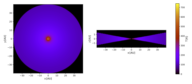
Consider the temperature gradient in the dust, and look up the minimum and maximum temperature values. As noted in the subsection about Output files above, the indicative dust temperature shown here does not correspond to a physical temperature, but rather reflects one of the many ways to obtain a representative temperature for a dust mixture.
PTS offers a simple way to create a plot of the spectral energy distributions (SEDs) produced by a SKIRT simulation. The SEDs for all instruments are combined on the same figure. After the simulation has completed, make sure that the output directory is your current directory, and enter the following command:
$ pts plot_seds . --prefix=PanTorus --dex=1.5 --wmin=0.1 --wmax=200
which includes these arguments:
plot_seds is the name of the PTS command to be performed.--prefix=PanTorus specifies the simulation to be handled (default is to handle all simulations in the directory).--dex=1.5 specifies the number of decades on the vertical flux axis of the plot.--wmin=0.1 and --wmax=200 specify the wavelength range on the horizontal axis, with values in micron.The contents of the generated PDF file should look like the plot at the start of this tutorial, i.e.:
It is obvious that the edge-on extinction is a lot stronger than the face-on extinction, as can be expected from the dust geometry. The effect is especially strong for shorter wavelengths because the dust grain cross sections are larger in that wavelength regime. The dust emission continuum in the (far-)infrared is isotropic because the dust is essentially transparent at those wavelengths.
Finally, open the instrument data cubes (PanTorus_i00_total.fits and PanTorus_i90_total.fits) in a FITS viewer and browse through the frames (or wavelengths). Manually adjust the range of the pixel values shown, clipping away the extremely bright central pixel. When comparing between frames, make sure to use the same scale and pixel range. To determine the wavelength corresponding to a particular frame index in the data cube, open one of the SED files (e.g. PanTorus_i00_sed.dat) in a text editor: the first column lists the wavelengths.
Interpret the results in the data cubes for each wavelength regime. Outside of the central pixel, the UV/optical radiation reaching the instruments has been scattered by dust grains in the torus. In the (far-)infrared, the dust grains re-emit the thermal energy absorbed at shorter wavelengths.
Congratulations, you made it to the end of this tutorial!