 |
The SKIRT project
advanced radiative transfer for astrophysics
|
|
The SKIRT project
advanced radiative transfer for astrophysics
|
In this tutorial you will work with a basic spiral galaxy model that includes the effects of polarization caused by the scattering of stellar radiation by spherical dust grains. You will discover a signature of the spiral arms in the polarization degree of the observed radiation, at least for this simplified model.
This tutorial assumes that you have completed the introductory SKIRT tutorials Monochromatic simulation of a dusty disk galaxy ad Panchromatic simulation of a dust torus, or that you have otherwise acquired the working knowledge introduced there. At the very least, before starting this tutorial, you should have installed the SKIRT code, and preferably also PTS and a FITS file viewer such as DS9 (see Installation Guide).
The polarization state of electromagnetic radiation is commonly described by the Stokes vector, the linear polarization degree and the polarization angle. For a brief recap of these concepts, see Configuring for polarized radiation. For a more extensive background and a description of the implementation of polarization in SKIRT, refer to Polarization by spherical grains in the developer guide.
To avoid spending time creating yet another SKIRT parameter file from scratch, this tutorial offers a ski file for download to serve as an initial configuration. Download the file TutorialPolarizationSpiral.ski using the link provided in the table below and put it into your local working directory.
| Initial SKIRT parameter file | TutorialPolarizationSpiral.ski |
|---|
Rename the downloaded SKIRT parameter file to a shorter name of your liking ending with the ".ski" filename extension, for example Spiral.ski. Run this ski file with SKIRT. If SKIRT immediately produces a fatal error while constructing the simulation, this probably means that the ski file needs upgrading; see Upgrading SKIRT parameter files.
While the simulation is running, open the ski file in a text editor and examine its contents. You should recognize the following configuration elements (not in this order):
MeanTrustBenchmarkDustMix, representing the dust properties used in the Gordon et. al 2017 benchmark (see Dust slab externally illuminated by a star)After the SKIRT simulation completes, examine its output. View the surface brightness frames generated by the instruments at various inclinations and wavelengths until you are satisfied that the results are as expected.
Enabling polarization in this configuration is straightforward. Duplicate the ski file and rename the copy, for example to PolarSpiral.ski. Open the new file in your text editor and make the following adjustments:
MeanTrustBenchmarkDustMix, change the value of the scatteringType option from "HenyeyGreenstein" to "SphericalPolarization";recordPolarization option from "false" to "true".Save these changes and run the updated ski file with SKIRT. Continue reading while the simulation is running.
As indicated in the introduction, SKIRT supports polarization of radiation by scattering on spherical dust grains. This feature is automatically enabled if the material mixture(s) in the configuration offer the appropriate optical properties (i.e., essentially, the Müller matrix that describes the changes to the Stokes vector during a scattering event). In that case, the radiation's polarization properties are tracked as photon packets move through the medium, and the instruments can be requested to record the components of the Stokes vector for detected photon packets, accumulated in each pixel/wavelength bin.
The MeanTrustBenchmarkDustMix class implements the relevant properties for a "representative grain" of the complete grain population, i.e. integrated over the size distribution and summed over material types. This is fine for a treatment of scattering in the optical range (as in this tutorial), but when including dust emission the calculation requires specific information for multiple grain size bins. See Configuring for polarized radiation for configuration options in this respect.
After the SKIRT simulation with polarization support completes, examine the output directory. For each instrument, there now are three extra FITS files containing the Stokes Q, U, and V components, in addition to the "totals" file containing the intensity (i.e. the Stokes I component).
Open the Q and U components for an instrument with face-on inclination in a FITS file viewer, and open an inspector showing a histogram of the pixel values (DS9->Scale->Parameters). In contrast to the intensity, the other Stokes components can have negative values. To enhance visualization of the spatial structure, you may need to play with the color bar scheme, scale and range. It might help to clip the values at zero (i.e. only showing positive values) to avoid problems with typical color scales such as the log scale.
Compare the 2D structure of the Q and U components. Examine the differences as you browse through the wavelengths.
While the Stokes components correspond to the output of an actual observation, it is much easier to interprete quantities such as the polarization degree and angle, which can be calculated from the Stokes vector components (see Describing the polarization state).
Using PTS, you can easily produce plots of polarization degree and angle for the output of a SKIRT simulation. To generate a default polarization map per instrument and per wavelength, simply enter (with the SKIRT output directory as the current directory):
pts plot_polarization . --bin=20
The bin argument specifies the number of image frame pixels (in each spatial direction) to be combined in a single "polarization" bin. Because of the limited number of photon packets launched for this tutorial, the output is fairly noisy, and it is best to specify fairly large bins (e.g. 20 by 20 pixels). If you rerun the simulation with substantially more photon packets, you might get acceptable plots with a reduced bin size.
This produces plots like these:
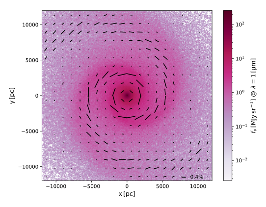
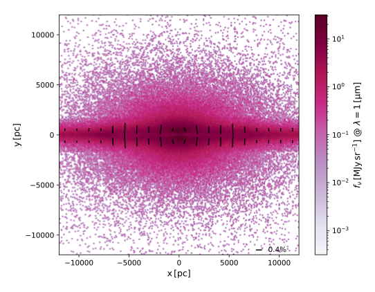
These figures show surface brightness maps (color scale) overlaid with linear polarization maps (line segments) for the spiral galaxy model of this tutorial, observed at a wavelength of \(1 \mu\mathrm{m}\). The orientation of the line segments indicates the polarization angle, and the size of the line segments indicates the degree of linear polarization. The top figure shows the model face-on, and the bottom figure shows the model edge-on.
The polarization degree is up to 1% around the central part of the model. In the face-on view, the orientation of the polarization is circular around the central bulge, showing a clear spiral structure. In the edge-on view, the polarization degree shows maxima at two positions to the left and two positions to the right of the center. When comparing with the face-on view, it appears that these positions correspond to the edge-on projection of the spiral arm structure.
The pts plot_polarization command can also generate other types of plots. For example, to plot the linear polarization degree averaged over the Y-axis per instrument and per wavelength, enter:
pts plot_polarization . --plot=degavg
The result is obtained by averaging each individual component of the Stokes vector over the Y-axis at each X position, and calculating the polarization degree from these totals. This produces plots like this one:
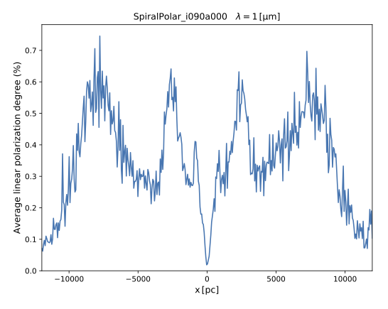
This average polarization degree plot corresponds to the edge-on polarization map shown above (i.e. they are for the same inclination and wavelength). Even if the two plots unfortunately do not have the same horizontal size, it is easily verified that the polarization degree maxima indeed occur at the same X-axis positions.
The model confguration for this tutorial includes a second set of instruments with lines of sight at the same inclinations but with a different azimuthal angle, resulting in a "rotated" view. The figure below shows adjacent results for the original view (left column) and for the rotated view (right column). This figure was produced by a custom Python script and is based on a simulation using many more photon packets (see Peest et al. 2017).
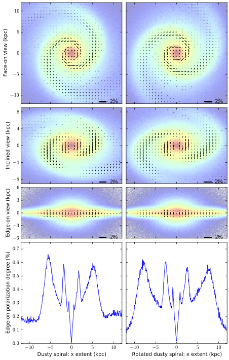
From this figure it is clear that regions with higher linear polarization trace the spiral arms at all inclinations, including the edge-on view. The maxima in the polarization signature of the edge-on view match the positions of the spiral arms along the line of sight. Indeed, the peaks in the polarization signature align with the tangent points of the spiral arms, which for the rotated view (right column) are farther out from the center of the galaxy.
These results imply that polarization measurements could be used, at least in principle, to study the spiral structure of edge-on spiral galaxies, where intensity measurements alone have limited diagnostic power.
Congratulations, you made it to the end of this tutorial!