The command scripts of the PTS visual package allow visualizing various SKIRT results by creating plots in PDF format or RGB images in PNG format. This page describes some of these commands with the objective to introduce the key concepts that are used by most of these visualization tools. For more details, see the reference documentation at pts.visual.do. Also, several of these commands are used as part of the tutorials.

Cuts and projections

The plot_density command script (pts.visual.do.plot_density) handles planar cuts through or projections of the source or medium density generated by a relevant SKIRT probe. It takes the following arguments:

simDirPath (positional string argument): the path to the SKIRT simulation output directory, or "." for the current directory
prefix (string): the prefix of the simulation to handle; by default handles all simulations in the directory
dex (float): if specified, the number of decades to be included in the density range (color bar); default is 5

For example, assume that the simulation introduced in the tutorial Stochastic heating in an SPH-simulated galaxy would be equipped with the following additional probes:

<DensityProbe probeName="dnscut" aggregation="Type" probeAfter="Run">
    <form type="Form">
        <DefaultCutsForm/>
    </form>
</DensityProbe>
<DensityProbe probeName="dnspro_xy" aggregation="Type" probeAfter="Run">
    <form type="Form">
        <ParallelProjectionForm inclination="0 deg" azimuth="0 deg" roll="90 deg"
                fieldOfViewX="4e4 pc" numPixelsX="1024" fieldOfViewY="4e4 pc" numPixelsY="1024"/>
    </form>
</DensityProbe>
<DensityProbe probeName="dnspro_xz" aggregation="Type" probeAfter="Run">
    <form type="Form">
        <ParallelProjectionForm inclination="90 deg" azimuth="-90 deg" roll="0 deg"
                fieldOfViewX="4e4 pc" numPixelsX="1024" fieldOfViewY="4e4 pc" numPixelsY="1024"/>
    </form>
</DensityProbe>
<DensityProbe probeName="dnspro_yz" aggregation="Type" probeAfter="Run">
    <form type="Form">
        <ParallelProjectionForm inclination="90 deg" azimuth="0 deg" roll="0 deg"
                fieldOfViewX="4e4 pc" numPixelsX="1024" fieldOfViewY="4e4 pc" numPixelsY="1024"/>
    </form>
</DensityProbe>

The output files generated by these probes can then be visualized with following PTS command:

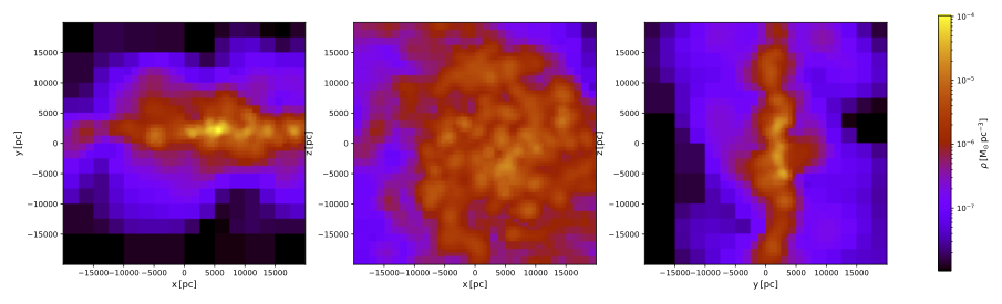
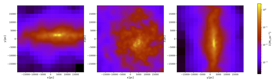
$ pts plot_dens . --prefix=PanEagle --dex 4
  Starting visual/plot_density...
  Created /Users/.../PanEagle_dnscut_dust_rho.pdf
  Created /Users/.../PanEagle_dnspro_dust_Sigma.pdf
  Finished visual/plot_density.

The PDF plot files are placed next to the simulation output file(s) being handled. The filenames include the simulation prefix, the probe name, a medium indicator ("dust"), and a physical quantity indicator ("rho" or "Sigma"). Furthermore, the command script has combined the three views called "xy", "xz" and "yz" in a single plot file. The DefaultCutsForm automatically conforms to the proper output file naming convention; for the ParallelProjectionForm the user can include the "xy", "xz" and "yz" at the end of the respective probe names.

$ open PanEagle_dnscut_dust_rho.pdf

$ open PanEagle_dnspro_dust_Sigma.pdf

Similar PTS command scripts can plot the cuts or projections produced by probes for opacity (pts.visual.do.plot_opacity), temperature (pts.visual.do.plot_temperature), velocity (pts.visual.do.plot_velocity) or magnetic field (pts.visual.do.plot_magnetic_field). Note that these command scripts also handle the output from input model probes, for example for the imported stellar mass density or imported medium density. For more information on probes, see Probes and forms.

RGB images

The make_images command script (pts.visual.do.make_images) creates RGB images in PNG format for the surface brightness maps produced by the instruments of a SKIRT simulation. The R,G,B color channels can be specified as wavelength values or as broadbands.

The script takes the following arguments:

simDirPath (positional string argument): the path to the SKIRT simulation output directory, or "." for the current directory.
prefix (string): the prefix of the simulation to handle; by default handles all simulations in the directory.
type (string): the final segment of the name of the instrument output files to be handled, excluding the ".fits" suffix (for example, "primaryscattered"); by default the script handles the "total" output files.
name (string): a name that will be added to the end of the image file name; defaults to the empty string.
colors (string): a string specifying the three wavelength values or broadbands corresponding to each R,G,B color channel of the image; by default the script uses frames with wavelengths as widely apart as possible.

The image files are placed next to the "*.fits" file(s) being represented, with the same filename but extended with the specified name string and the filename extension replaced by ".png".

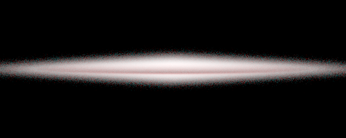
For example, after running a panchromatic simulation of a basic spiral galaxy model with a substantial amount of dust, one could create the following images:

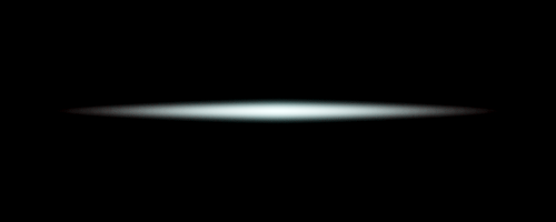
$ pts make_images . --name=optical --colors="SDSS_Z,SDSS_R,SDSS_U"
  Starting visual/make_images...
  Convolving for RGB image diskemi_i88_total_optical
  Created convolved RGB image file /Users/.../diskemi_i88_total_optical.png
  Finished visual/make_images.
$ pts make_images . --name=fir --colors="PACS_160,PACS_100,PACS_70"
  Starting visual/make_images...
  Convolving for RGB image diskemi_i88_total_fir
  Created convolved RGB image file /Users/.../diskemi_i88_total_fir.png
  Finished visual/make_images.
$ open diskemi_i88_total_optical.png

$ open diskemi_i88_total_fir.png

Spectra

The plot_seds command script (pts.visual.do.plot_seds) creates plots of the SEDs produced by the instruments of a SKIRT simulation.

The script takes the following arguments:

simDirPath (positional string argument): the path to the SKIRT simulation output directory, or "." for the current directory
prefix (string): the prefix of the simulation to handle; by default handles all simulations in the directory
instr (string): the name of the instrument to handle; by default handles all instruments in the simulation
wmin (float): smallest wavelength on the horizontal axis, in micron; default is 0.1 micron
wmax (float): largest wavelength on the horizontal axis, in micron; default is 1000 micron
dex (float): if specified, the number of decades to be plotted on the vertical axis; default is 5

The plot files are placed next to the "*_sed.dat" file(s) being represented. The filename starts with the simulation prefix and ends with "sed.pdf". If there are multiple SED instruments in the simulation, the plot shows the total flux for each instrument. If there is just a single instrument, or if an instrument was specified using the instr argument, the plot shows the total flux in addition to the transparent flux and the primary and secondary flux components.

For examples, see Spectra in the tutorial Stochastic heating in an SPH-simulated galaxy.