To estimate the intensities of emission or absorption lines for atomic and molecular transitions under non-local thermodynamic equilibrium (non-LTE) conditions, it is crucial to self-consistently calculate both the energy level populations and the radiation field. SKIRT performs these self-consistent calculations, allowing for the accurate estimation of emission or absorption lines for selected transitions, given a spatial gas distribution and a background radiation. This page describes how to configure such SKIRT simulations.

The ski file offered for download here is a fully configured example. It is not intended to be executed "as is" because the required input files are not available. However, it will serve as a helpful reference during the discussion on this page.

Example SKIRT parameter file	NonLTELines.ski

Additional reading:

The NonLTELineGasMix class documentation lists the supported transitions and species.
The web page Non-LTE line radiative transfer in a sphere discusses the SKIRT results for the van Zadelhoff et al. 2002 benchmark, a basic but relevant application of the concepts discussed here, and offers the related ski files for download.
Matsumoto et al. 2023 (A&A, 678, A175) describe the implementation of the atomic/molecular line calculations in SKIRT and present a study using them.

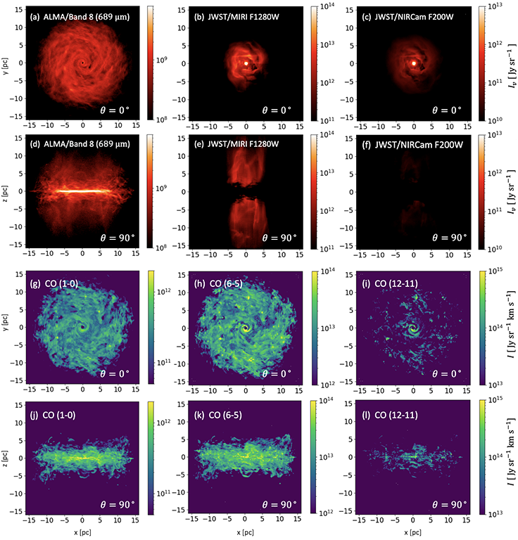
Dust continuum and CO line emission maps for the AGN torus model discussed in Matsumoto et al. 2023.

Introduction

A SKIRT simulation that calculates atomic/molecular lines must include at least one medium component that is associated with the NonLTELineGasMix material mix. The NonLTELineGasMix class configuration selects one of the supported species. The medium component then defines the spatial distribution of the relevant properties, including the number density of the species under consideration and kinematic information such as temperature and bulk velocity. Most often, this information will be read from an input file by associating the NonLTELineGasMix with a subclass of ImportedMedium.

A simulation that includes a gas species represented by the NonLTELineGasMix requires one or more primary sources that directly trigger energy transitions (e.g., the cosmic microwave background). Additionally, the simulation may incorporate a dust medium to estimate dust emission, which can also excite these energy transitions. In any case, the calculation requires iteration to obtain a converged result that is self-consistent with the gas medium's own line emission. During a given iteration in the simulation, the emission luminosity and absorption opacity for each supported transition are determined in each cell from the medium properties and the local radiation field calculated by the simulation.

The simulation's radiation field wavelength grid should therefore properly resolve the relevant emission line profiles as well as the continuum radiation resulting from primary and secondary sources. To avoid a prohibitively large number of grid points, this requires two levels of spectral resolution: a moderate resolution covering the full wavelength range considered in the simulation, and a much higher resolution covering each of the narrow line profiles. These two levels of resolution must be merged into a single radiation field wavelength grid. In contrast, multiple instruments can be configured for distinct wavelength ranges of interest. For example, the complete continuum spectrum can be covered by an instrument using a regular logarithmic grid, and each line profile can be covered by its own separate instrument using a linear grid.

Finally, to boost performance, SKIRT must be told to favor photon packet wavelengths in the narrow ranges around the line profiles over those in the overall continuum.

The following sections address more concrete configuration guidelines for these various issues.

Note: While we provide suggestions for the values of several configuration parameters, it is important to run test simulations for a representative model in your study with varying parameter values until the simulated observables are properly converged.

Experience level

When configuring your first simulation of this type using the command line Q&A or the Makeup wizard, select user experience level "Regular" and configure straightforward, built-in wavelength grids. Expert options and complex wavelength grids can be adjusted or added later by manually editing the ski file.

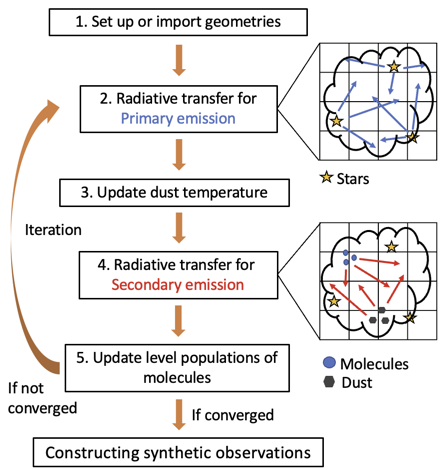
Simulation mode and iteration options

A simulation of this type proceeds in two phases: primary emission and secondary emission.

During primary emission, the simulation determines the radiation field resulting from the primary sources, dust attenuation and atomic/molecular line absorption based on their level populations. Initially, the level populations are determined under LTE conditions, assuming no radiative transitions. However, after the calculation of the radiation field induced by primary emission, an improved estimate of the level populations for each spatial cell is made, taking both collisional and radiative transitions into account.

During secondary emission, the simulation takes into account emission from all configured media, including atoms, molecules, and dust, in addition to absorption by these same media. Emission line profiles and line absorption cross sections are determined from the previously stored level populations. Similarly, dust heating and emission is determined from the previously stored radiation field. This secondary emission phase establishes an updated radiation field, which is used to update the level populations. However, the updated radiation field and level populations in turn influence the line emission/absorption profiles and the dust heating/emission. The simulation must therefore perform iterations over secondary and possibly primary emission to obtain a self-consistent result.

This leads to the following configuration requirements/recommendations:

simulationMode must be set to "DustAndGasEmission" if the simulation includes dust or to "GasEmission" if it does not.
iteratePrimaryEmission (an expert option, disabled by default) should be enabled only in the rare case iteration is required for other media (for example, to self-consistently calculate radiative dust destruction).
iterateSecondaryEmission must be enabled.
includePrimaryEmission (an expert option, disabled by default) should be enabled only if the wavelength range of the primary source(s) significantly overlaps the emission lines of the species under consideration; in other words, if the opacity at the line wavelengths significantly affects the primary radiation field through absorption. For example, when simulating sub-millimeter lines (e.g., CO, HCO+, etc.), the CMB radiation overlaps with the wavelengths of the emission lines. Therefore, this option must be enabled.
minSecondaryIterations can be left at the default value of 1.
maxSecondaryIterations most likely needs to be increased substantially from the default value of 10 to 50 or more, depending on the configured convergence criteria (see below) and the convergence behavior of the simulated model.

Convergence criteria

The NonLTELineGasMix class offers options to configure the convergence criteria that determine when the iterative calculation terminates. The first two properties configure a criterion based on statistics per spatial cell, while the third property configures a global criterion. Both criteria must be satisfied simultaneously:

maxChangeInLevelPopulations specifies the maximum relative change between consecutive iterations in the level populations for a given spatial cell for that cell to be considered converged.
maxFractionNotConvergedCells specifies the maximum fraction of spatial cells (relative to the total number of spatial cells in the simulation) that may be left not converged for the whole spatial domain to be considered converged.
maxChangeInGlobalLevelPopulations specifies the maximum relative change between consecutive iterations in the global level populations, accumulated over the complete spatial domain, for the spatial domain to be considered converged.

Note: A parameter similar to maxChangeInLevelPopulations is used in many other non-LTE line radiative transfer codes. We recommend specifying a loose value (0.1-1.0) for maxChangeInLevelPopulations and applying a stricter value for maxChangeInGlobalLevelPopulations (0.01). This is because, in our Monte Carlo-based calculations, Monte Carlo noise can interfere with the convergence of the local level distribution.

If the simulation includes dust, the DustEmissionOptions include properties to configure the convergence criteria for dust self-absorption and heating:

maxFractionOfPrimary: convergence is reached when the total absorbed dust luminosity is less than this fraction of the total absorbed primary luminosity.
maxFractionOfPrevious: convergence is reached when the total absorbed dust luminosity has changed by less than this fraction compared to the previous iteration.

It is recommended to start with the default values for all convergence criteria and adjust them based on initial simulation results. For dust self-absorption, the defaults will suffice unless the dust opacity is very high. For the level populations, chances are that the defaults need to be adjusted. The objective is to obtain an acceptable balance between execution time (number of iterations) and accuracy of the simulated observables.

Spatial distribution of medium properties

The NonLTELineGasMix material mix is often associated with a subclass of ImportedMedium. This allows reading the spatial distribution of the relevant medium properties from an input file, possibly exported from a hydrodynamical simulation snapshot. The input file must provide values for the spatial distribution of the number density of the species under consideration, the number density of any relevant collisional partner species, the kinetic gas temperature, and the turbulence velocity. It will often also include values for the spatial distribution of the bulk velocity. Once imported, all of these values remain constant during the simulation.

It is important to set the options in the ImportedMedium component appropriately as follows:

massType: set to "NumberDensity".
massFraction: leave at the default value of 1 unless the number density given in the input file must be reduced by a fixed factor.
importMetallicity: leave at the default value of "false".
importTemperature: set to "true" (!!).
maxTemperature: leave at the default value of 0 K.
importVelocity: set to "true" if the input file incudes bulk velocity components, "false" otherwise.
importMagneticField (an expert option): leave at the default value of "false".
importVariableMixParams: leave at the default value of "false".

The additional columns required by the material mix are automatically imported and are expected after all other columns. For example, if bulk velocities are also imported for this medium component, the column order would be

$. . ., n_{m o l}, T_{k i n}, v_{x}, v_{y}, v_{z}, n_{c o l 1} [, n_{c o l 2}, . . .], v_{t u r b}$

In this case, the NonLTELineGasMix options specifying default values for input data (defaultTemperature, defaultCollisionPartnerRatios, defaultTurbulenceVelocity) are not used because this information is read from the input file. It is best to leave these options at their respective default values.

On the other hand, for basic testing purposes, the NonLTELineGasMix can also be associated with a geometric medium component. The geometry then defines the spatial density distribution of the species under consideration (i.e. $n_{m o l}$ ), and the NonLTELineGasMix configuration properties specify a fixed default value for the other properties that will be used across the spatial domain. The number densities of the collisional partners are now defined by a constant multiplier relative to $n_{m o l}$ as opposed to an absolute value.

Radiation field wavelength grid

The simulation's radiation field wavelength grid must properly resolve the relevant emission line profiles as well as the continuum radiation resulting from primary and secondary sources. To avoid a prohibitively large number of grid points, this requires two levels of spectral resolution and thus a custom wavelength grid with precisely placed bins. While the appropriate values could be entered during the Q&A session, it is far easier to automate this process through a simple Python script. One option is to produce a file with the required wavelength points and use the FileWavelengthGrid class to build the corresponding grid. A nice alternative is to employ the CompositeWavelengthGrid class to combine a set of separately configured wavelength grids into a single grid. This explicitly documents the makeup of the grid in the ski file and avoids the need for a seperate input file.

For example, the following composite wavelength grid covers a continuum range with 100 bins, plus three line profiles with 50 bins each:

<CompositeWavelengthGrid log="false">
    <wavelengthGrids type="DisjointWavelengthGrid">
        <LogWavelengthGrid minWavelength="0.01 micron" maxWavelength="30 micron" numWavelengths="100"/>
        <LinWavelengthGrid minWavelength="2600.541 micron" maxWavelength="2600.975 micron" numWavelengths="50"/>
        <LinWavelengthGrid minWavelength="1300.301 micron" maxWavelength="1300.518 micron" numWavelengths="50"/>
        <LinWavelengthGrid minWavelength="866.8851 micron" maxWavelength="867.0297 micron" numWavelengths="50"/>
    </wavelengthGrids>
</CompositeWavelengthGrid>

This ski file snippet, or at least the portion covering the line profiles, could be automatically generated by a script and then hand-copied into the ski file. Note that the various subgrids are allowed to overlap, although this is not the case in the example above.

The continuum portion of this wavelength grid is only required for calculating dust heating and emission. We expect the radiation field at shorter wavelengths to dominate the dust heating process, with the longer wavelengths having a minimal effect. We can also presume that the precise wavelength of an incoming photon packet is not so important as long as its energy is properly categorized, thus allowing fairly wide wavelength bins. Experiments have shown that for a typical (simulated) spiral galaxy, a grid ranging from 0.02 to 10 micron with 40 bins is sufficient. The short end of the range must be extended accordingly for models with sources emitting at shorter wavelengths. The long end of the range must be extended for models with high dust optical depth, because the dust heating process may be affected by longer wavelengths.

The high-resolution portions of this wavelength grid should be sufficiently wide to cover the corresponding line profiles, and not wider to avoid wasting computation time and memory. The local radiation field in each spatial cell is calculated in the rest frame of the medium in that cell. Therefore, it suffices to cover a gaussian profile broadened by thermal and microturbulence. A reasonable range seems to be 5 times the maximum microturbulence in the simulation on each side of the central line wavelength. The example above uses $\pm 25 k m / s$ .

Primary sources

The SourceSystem wavelength range determines the maximum range in which any source can radiate. This range is configured through the SourceSystem minWavelength and maxWavelength properties (the wavelengths property is not used in panchromatic simulations). Specifically, the wavelength range in which a given source will be emitting is determined by the intersection of the range over which the source's SED is defined and the SourceSystem wavelength range.

On a side note, when configuring the IntegratedLuminosityNormalization for a given source, one must specify a wavelength range. To avoid confusion, it is best to select the "Custom" option for the wavelengthRange property and then use the minWavelength and maxWavelength properties to specify the range. While this determines the spectral range of the integration involved in the normalization, it does not affect the range over which the source will be emitting.

Dust emission

If the simulation includes dust, the dust emission wavelength grid controls the resolution of the dust emission spectrum calculated for each spatial cell. It is configured through the DustEmissionOptions option dustEmissionWLG.

Especially when taking into account the stochastic heating of small dust grains, this spectrum contains many narrow infrared features. It is thus desirable to configure a grid that can properly resolve these features. Memory usage is not an issue because the emission spectrum is stored just once per execution thread. The performance impact is very limited as well because sampling these emission spectra is not the bottleneck of the calculation. On the other hand, because the dust emission spectrum is essentially constant across the width of a transition line, there is no need to have the dust emission wavelength grid resolve the line profiles considered in the simulation.

One could employ a NestedLogWavelengthGrid with a resolution of 100 bins per dex in the overall range from 0.2 to at least 2000 micron, and 200 narrower bins in the range from 3 to 25 micron, for a total of just over 500 bins. Even if the wavelength range of all instruments and probes is smaller, it is still important to configure a dust emission wavelength grid with this full spectral range for the dust emission calculations to be correct.

Wavelength bias distribution

According to the Monte Carlo principle, when launching a photon packet, SKIRT should randomly sample its initial wavelength from the SED of the source. However, this would cause many photon packets to be concentrated in high-luminosity spectral ranges, leaving ranges with lower luminosity poorly sampled. SKIRT therefore samples a fraction of the initial wavelengths from a "bias distribution", adjusting the relative photon packet weights to compensate. By configuring the bias distribution of a source (an expert option), a user can cause a larger fraction of photon packets to be launched in spectral ranges that need to be sampled more extensively, at the expense of poorer sampling in other ranges.

By default, SKIRT samples half of the initial wavelengths from the source SED, and the other half from a regular logarithmic distribution. For the majority of simulations, this provides a good balance between favoring high-luminosity ranges and acceptable sampling in low-luminosity ranges. For simulations with self-consistent line calculations, however, it is beneficial to force a more substantial fraction of the initial wavelengths to be inside the line profile ranges.

To configure the wavelength bias distribution for a source, one could enter the appropriate choices and values during the Q&A session. As discussed in the section on the radiation field wavelength grid, it is far easier to automate this process through a simple Python script. One option is to produce a file tabulating the required probability distribution and use the FileWavelengthDistribution class to import this file. A nice alternative, however, is to employ a trick that allows piggy-backing on the method described for the radiation field wavelength grid, based on the CompositeWavelengthGrid class.

The DiscreteWavelengthDistribution class was originally designed for a different purpose, but it comes in handy here. The class derives a discrete wavelength probability distribution from an arbitrary wavelength grid configured by the user. Specifically, it will select the initial photon packet wavelengths from the central wavelengths of the configured grid, with equal probability. Combined with the CompositeWavelengthGrid class, this can be used to construct a bias distribution that specifies discrete wavelengths across a given set of line profiles, as shown in the examples below. It may seem weird to use a distribution that launches photon packets at a set of specific wavelength values rather than at a continuous range of values. This is not really a problem here because the wavelengths are Doppler-shifted anyway as a result of the model kinematics. Also, the user can specify that a fraction of wavelengths should still be sampled from the source SED as usual.

For example, the following ski file snippet would define a background source with a wavelength bias distribution for three line profiles. Because the background radiation does not noticably affect the dust heating, there is no need to launch photon packets outside of the line profile ranges, so that the wavelengthBias property can be set to 1.

<CubicalBackgroundSource ... wavelengthBias="1">
    <sed type="SED">
        <BlackBodySED temperature="2.725 K"/>
    </sed>
    <normalization type="LuminosityNormalization">
        <IntegratedLuminosityNormalization wavelengthRange="Custom" minWavelength="100 micron" maxWavelength="3000 micron" .../>
    </normalization>
    <wavelengthBiasDistribution type="WavelengthDistribution">
        <DiscreteWavelengthDistribution>
            <wavelengthGrid type="DisjointWavelengthGrid">
                <CompositeWavelengthGrid log="false">
                    <wavelengthGrids type="DisjointWavelengthGrid">
                        <LinWavelengthGrid minWavelength="2599.456 micron" maxWavelength="2602.059 micron" numWavelengths="150"/>
                        <LinWavelengthGrid minWavelength="1299.759 micron" maxWavelength="1301.060 micron" numWavelengths="150"/>
                        <LinWavelengthGrid minWavelength="866.5236 micron" maxWavelength="867.3911 micron" numWavelengths="150"/>
                    </wavelengthGrids>
                </CompositeWavelengthGrid>
            </wavelengthGrid>
        </DiscreteWavelengthDistribution>
    </wavelengthBiasDistribution>
</CubicalBackgroundSource>

Note that the wavelength grids covering the line profiles now need to be sufficiently wide to also capture kinematic broadening. A reasonable starting point is to extend the range on each side of the central line wavelength by the largest bulk velocity in the simulation, in addition to 5 times the largest microturbulence. The example above uses $\pm 200 k m / s$ . The example also specifies a larger number of grid points (150 points compared to the 50 bins in the radiation field wavelength grid) to improve sampling of the emission spectrum and kinematic effects.

The same simulation model might include a point source emulating an active galactic nucleus. Because the spectrum of this source does not overlap the line profiles considered in the simulation, the default bias distribution is fine.

<PointSource ... wavelengthBias="0.5">
    ...
    <sed type="SED">
        <FileSED filename="AGN_SED.txt"/>
    </sed>
    <normalization type="LuminosityNormalization">
        <IntegratedLuminosityNormalization wavelengthRange="Custom" minWavelength="0.001 micron" maxWavelength="32 micron" ..."/>
    </normalization>
    <wavelengthBiasDistribution type="WavelengthDistribution">
        <LogWavelengthDistribution minWavelength="1e-6 micron" maxWavelength="1e6 micron"/>
    </wavelengthBiasDistribution>
</PointSource>

Dust emission must also be configured with a wavelength bias distribution. Optionally including the same NestedLogWavelengthGrid as the one configured for calculating the emission spectrum helps favoring the spectral range with detailed dust features. In any case, the wavelengthBias property should be left at the default value of 0.5 to ensure that the regular dust spectrum is sampled as well.

<DustEmissionOptions dustEmissionType="Stochastic" ... wavelengthBias="0.5">
    ...
    <dustEmissionWLG type="DisjointWavelengthGrid">
        <NestedLogWavelengthGrid ..."/>
    </dustEmissionWLG>
    <wavelengthBiasDistribution type="WavelengthDistribution">
        <DiscreteWavelengthDistribution>
            <wavelengthGrid type="DisjointWavelengthGrid">
                <CompositeWavelengthGrid log="false">
                    <wavelengthGrids type="DisjointWavelengthGrid">
                        <NestedLogWavelengthGrid .../>
                        <LinWavelengthGrid minWavelength="2599.456 micron" maxWavelength="2602.059 micron" numWavelengths="150"/>
                        <LinWavelengthGrid minWavelength="1299.759 micron" maxWavelength="1301.060 micron" numWavelengths="150"/>
                        <LinWavelengthGrid minWavelength="866.5236 micron" maxWavelength="867.3911 micron" numWavelengths="150"/>
                    </wavelengthGrids>
                </CompositeWavelengthGrid>
            </wavelengthGrid>
        </DiscreteWavelengthDistribution>
    </wavelengthBiasDistribution>
</DustEmissionOptions>

Finally, for the NonLTELineGasMix line emission, the wavelength bias distribution is ignored so it can be left at the default. The wavelengthBias property should be set to 1, specifying that photon packet launches will be distributed equally between all lines (as opposed to taking into account the relative line luminosities).

<NonLTELineGasMix ... wavelengthBias="1" ...>
    <wavelengthBiasDistribution type="WavelengthDistribution">
        <LinWavelengthDistribution minWavelength="1e-6 micron" maxWavelength="1e6 micron"/>
    </wavelengthBiasDistribution>
</NonLTELineGasMix>

Instrument wavelength grids

Each instrument can be configured with its own distinct wavelength grid. It is often convenient to provide multiple instruments for a given line of sight rather merging everything into a single instrument. The performance impact of doing so is limited as long as instruments with the same line of sight are placed consecutively in the ski file.

Here are some examples of instrument/wavelength grid combinations that may be useful in this context:

an SEDInstrument with a high-resolution LogWavelengthGrid (1000 grid points or more) covering the complete combined wavelength range of the primary and secondary sources in the simulation, for recording the overall spectrum.
a FrameInstrument with a BandWavelengthGrid (pre-defined or configurable) for recording a set of broadband images.
an SEDInstrument with a high-resolution LinBorderWavelengthGrid (50 points or more) covering the line profile for one of the transitions studied in the simulation.
a FrameInstrument with a limited-resolution LinBorderWavelengthGrid (say 10 bins or so) covering the line profile for one of the transitions studied in the simulation. The grid might need to include a few bins adjacent to the line profile to allow estimating of the background continuum radiation.

In the latter two cases, a separate instrument can be configured for each transition, or multiple line profiles can be combined into a single wavelength grid using the CompositeWavelengthGrid. Note that the wavelength grids covering the line profiles need to be sufficiently wide to capture kinematic as well as thermal broadening (see the discussion of wavelength bias distributions above). Again, it is usually desirable to generate the relevant ski file snippets automatically through a Python script.