 |
The SKIRT project
advanced radiative transfer for astrophysics
|
|
The SKIRT project
advanced radiative transfer for astrophysics
|
Path length stretching (PLS) is an optimization (variance-reduction) technique used in Monte Carlo radiative transfer simulations to help photon packets efficiently traverse regions of higher optical depth. It is implemented in SKIRT and exposed through the pathLengthBias property of the PhotonPacketOptions in the ski file. The technique has side effects that cause it to be less desirable (or even not applicable) in certain simulation regimes.
This topic investigates the merits and limitations of PLS as it is implemented in SKIRT. If you're only interested in the final conclusions, skip to Summary at the end.
In the forced-scattering photon life cycle (see Configuring the photon packet life cycle), the optical depth \(\tau\) at which the next interaction occurs is normally drawn from the physical exponential distribution \(p(\tau)=\text{e}^{-\tau}\), truncated to the total optical depth \(\tau_\text{path}\) along the photon packet's path through the model. This distribution is strongly peaked towards small \(\tau\), so that interaction points deep inside an optically thick region are exceedingly rare: for example, a random optical depth beyond \(\tau=20\) occurs only about once in 485 million draws. Probing such regions with an unbiased Monte Carlo method therefore requires a very large number of photon packets.
PLS addresses this by sampling \(\tau\) from a shallower, artificial exponential distribution instead, and compensating for the bias with a corresponding weight factor on the photon packet. Pushed too far, however, this shift can itself introduce excessively large weight factors, trading one source of noise for another. Baes et al. (2016) resolve this trade-off with composite biasing: rather than replacing the physical pdf outright, the biased pdf used to draw \(\tau\) is a weighted combination of the physical distribution and the stretched one, with a mixing parameter \(\xi\in[0,1]\) that sets the fraction of path lengths effectively drawn from the stretched distribution. In the SKIRT implementation, the user can control the value of \(\xi\) through the pathLengthBias property of PhotonPacketOptions.
Because forced scattering already limits \(\tau\) to the finite range \([0,\tau_\text{path}]\), SKIRT combines the physical distribution with a uniform distribution over that same range, leading to the biased pdf
\[ q(\tau) = (1-\xi)\,\frac{\text{e}^{-\tau}}{1-\text{e}^{-\tau_\text{path}}} + \frac{\xi}{\tau_\text{path}} \qquad 0\le\tau<\tau_\text{path} \]
and the corresponding weight factor
\[ w(\tau) = \frac{p(\tau)}{q(\tau)} = \frac{1}{(1-\xi) + \xi\left(\dfrac{1-\text{e}^{-\tau_\text{path}}}{\tau_\text{path}}\right) \text{e}^{\tau}}, \]
which never exceeds \(1/(1-\xi)\), however large \(\tau_\text{path}\) becomes.
There are important caveats, however. Although the bias weight for a single scattering event is bounded to \(1/(1-\xi)\), multiple consecutive scattering events may still lead to large combined bias factors on some photon packets. See High albedo for a regime where this becomes problematic. At the other end of the bias scale, the applied bias weight might be so small that the contribution of the photon packet becomes negligible. Such photon packets get killed prematurely at the cutoff luminosity controlled by the minWeightReduction property of PhotonPacketOptions. See High optical depth for a regime where this becomes problematic.
SKIRT does not implement PLS when forced scattering is disabled (by setting the forceScattering property of PhotonPacketOptions to 'false'). The main benefit of the non-forced-scattering photon life cycle is that the optical depth for each path segment is calculated only up to the next interaction point, without the need for determining the optical depth along the full path to the edge of the model, thus significantly increasing performance for simulations with very short free paths between frequent scattering events. But because the optical depth of the full path is unknown, it is not possible to derive a meaningful alternative, stretched distribution that could be used to sample the interaction optical depth in the PLS technique.
The standard yardstick for judging whether a variance-reduction technique such as PLS is actually worthwhile is the figure of merit, \(\text{FOM}=1/(R^2\,T)\), where \(R\) is a measure for the error (Monte Carlo noise) of the quantity being estimated and \(T\) is the computation time needed to obtain it. A technique that reduces the noise but adds substantial overhead or requires many more photon packets may not actually improve the figure of merit; one that reduces the noise at negligible extra cost clearly does.
SKIRT supports the calculation of the figure of merit for the output of its instruments by tracking the relevant higher-order moments of the flux contributions in each bin. This option is enabled for a given instrument by setting the recordStatistics property of the instrument to 'true'. The topic Reliability statistics for simulated fluxes describes this feature in detail.
In this topic, we use the FOM measure to help us evaluate the PLS technique in various simulation regimes.
|
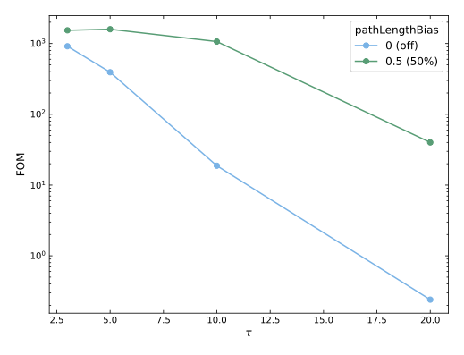
This plot shows the figure of merit (FOM) on an arbitrary scale (larger is better) as a function of optical depth, for a simulation that tracks the light penetrating through a slab of dust with uniform density. The configuration is borrowed from the TRUST benchmark Gordon et al. (2017) and is also used as an example in the SKIRT 9 paper Camps and Baes (2020). It is summarized as well in this user guide in Example: radiation penetrating thick slab.
The horizontal axis of the figure indicates the optical depth across the slab between the radiation source and the observer. Given the dimensions of the slab, the most extreme optical depth that would be seen by a photon packet scattered along the diagonal is nearly 5 times higher than the transverse optical depth.
At the single wavelength used in the simulation, the slab material has an albedo of 0.46, which means that about half of the photon packet energy is lost to absorption in each interaction (because SKIRT employs the scattering/absorption split technique that simulates both an absorption and scattering event at each interaction site). The scattering phase function is approximated by the "standard" Henyey-Greenstein function with an asymmetry parameter of 0.25, slightly favoring the forward direction in scattering events.
The figure clearly shows that, in this regime, the PLS technique offers a significant benefit to the simulation's performance. This is the "comfort zone" of the technique: low to mid-range optical depths and significant absorption relative to scattering. This regime includes, for example, the typical models of dusty galaxies that have been – and to some extent still are – the dominant application for SKIRT.
|
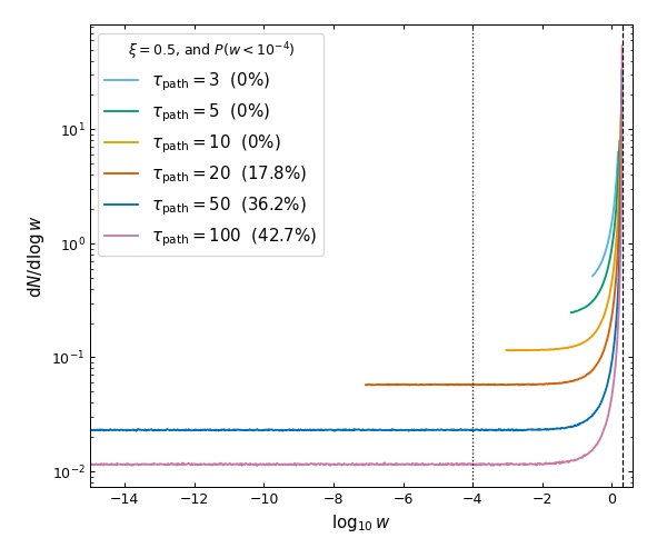
Although PLS was designed to more easily penetrate regions of high optical depth, the technique gets into trouble if the optical depth becomes too high. Even obtaining properly converged FOM values is hard because the simulation runtimes quickly become prohibitive. Instead, the figure above shows the probability distribution of the bias factor applied by PLS with \(\xi=0.5\) (the default value of the pathLengthBias property) for \(\tau_\text{path}\) up to 100.
To avoid spending time on photon packets with a negligible contribution to the end result, SKIRT aborts a photon packet as soon as its cumulative bias weight becomes smaller than a given threshold. This cutoff threshold is set through (the inverse of) the minWeightReduction property of PhotonPacketOptions, which has a default value of \(10^4\). Assuming this default cutoff threshold, the legend of the figure above shows that 18% of the interaction points sampled for paths with \(\tau_\text{path}=20\) will cause the packet under consideration to be aborted. For \(\tau_\text{path}=100\), the abort probability becomes 43%, and for \(\tau_\text{path}=1000\) (not shown in the figure) it already is at 49%, near the theoretical limit of 50%.
These numbers represent the abort rate for the first interaction. In practice, because packets are forced to interact multiple times during their lifetime, the compound multi-interaction rejection probability because of PLS can become exceedingly high. As a result, a simulation must launch a very large number of photon packets to generate a sufficient number of packets that properly sample the model, making the PLS technique largely ineffective in a regime with optical depths well above 20.
It should be noted that the slab model forces photon packets to fully travel through the transverse optical depth before being observed. In many models photon packets can "escape" the region of high optical depth as a result of the geometry (e.g. a planetary dust disk observed away from the edge-on sight line) or because of wavelength shifts (e.g. resonant scattering). In those configurations, the local optical depth can be much higher than the numbers shown/quoted above without adversely affecting the photon cycle or the PLS technique.
|
|
As mentioned in The comfort zone, SKIRT uses the scattering/absorption split technique. For each interaction, a bias weight is applied to the photon packet corresponding to the albedo of the medium, effectively mimicking the effect of absorption at the interaction site. In a medium with significant absorption, a packet "naturally" hits the cutoff threshold after a number of interactions. For media with little or no absorption, this is no longer the case. The only factor limiting a packet's lifetime is the "escape fraction", yet another bias weight representing the portion of the packet that would have left the model if it were not forced to scatter.
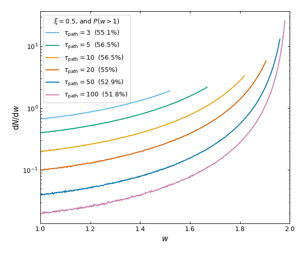
As a result, scattering-dominated media with a non-trivial optical depth present a challenge of a different nature to the PLS technique. The left panel of the figure above again shows the probability distribution of the bias weight applied by PLS with \(\xi=0.5\) for \(\tau_\text{path}\) up to 100, but now focusing on the portion with a weight larger than 1. By design, the weight is never above 2 (see The path length stretching technique). However, as listed in the legend, for all optical depths, slightly over 50% of the sampled weights are above 1. Repeated application might lead to large cumulative bias factors on some "lucky" photon packets.
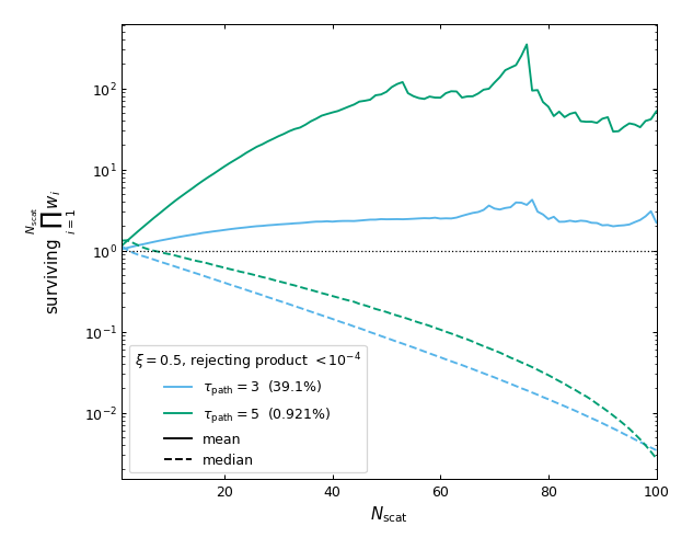
To illustrate this further, the right panel of the figure above shows the mean (solid curves) and median (dashed curves) accumulated bias weight for a photon packet as a function of the number of consecutive scattering events, assuming that any photon packet that dips under the threshold is aborted (and thus no longer takes part in the statistics). The plot also assumes that only the PLS bias weights affect the photon packets, approximating a medium that is strongly dominated by scattering and has a fair optical depth.
As expected, the median accumulated bias weight drifts steadily down as the number of scatterings increases. For most photon packets, the very small PLS bias weights win from those above 1 and pull the accumulated product down. However, some packets get an extremely lucky run of large weight draws and reach very large products. Those rare packets strongly pull up the mean accumulated product. Even if they are outliers, they do cause serious trouble as we will see next.
On a side note, as listed in the figure's legend, for \(\tau_\text{path}=3\) only 39% of the launched photon packets make it to 100 scattering events. For \(\tau_\text{path}=5\) this has decreased to less than 1%, and for \(\tau_\text{path}=10\) (not shown in the figure) only 1 out of 4 million packets reach the finish.
|
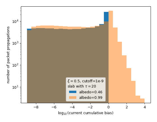
To produce the above figure, SKIRT was equipped with temporary instrumentation to log information at the start of each leg of the photon packet life cycle, i.e. just after emission and just after each scattering event. The figure shows results for two simulations of the slab configuration presented above in The comfort zone. The only difference between the simulations is the albedo of the medium: roughly half in one simulation, and essentially one (i.e. scattering-only) in the other.
The histograms show the unnormalized distribution of the photon packet's cumulative bias weight at the time of logging. The cutoff threshold was set to \(10^{-9}\) (in an unsuccessful attempt to improve the efficiency), and evidently there are no values to the left of this cutoff in the figure. For the simulation with albedo 0.46, there are no cumulative weights above 1 because the absorption bias at each interaction compensates for a potential increase. For the simulation with albedo 0.99, the cumulative bias weight for some photon packets rises up to a value of \(10^4\). These "boosted" packets contribute huge, unrealistic flux peaks in the simulated observables, significantly increasing noise and decreasing the corresponding FOM.
In conclusion, the PLS technique does not apply well to scattering-dominated media.
|
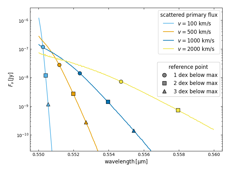
To study the behavior of PLS in moving media, we use a model consisting of an expanding spherical shell (inner radius 0.05 pc, outer radius 1 pc, density power-law exponent 0.5) around a central, stationary, isotropic point source emitting at a single wavelength of 0.55 micron. The shell material has the same optical properties as those used in The comfort zone, i.e. an albedo of 0.46 and a scattering asymmetry parameter of 0.25 (both values are approximate because the photon wavelength varies slightly as a result of kinematic effects). The shell density is normalized to a radial optical depth of 5 (or 10 along a full axis through the origin). The material moves radially outward so that within the shell the local outflow speed ramps up from about 22% of the configured velocity magnitude at the inner edge to 100% of it at the outer edge. This nominal velocity is varied over 100, 500, 1000 and 2000 km/s in separate simulations.
Because the source sits at the shell's centre, every photon's pre-scattering direction is exactly radial, i.e. co-moving with the local outflow at the point where it scatters. This means that the first scattering event can never blueshift the photon, which is why every curve in the figure above lies entirely redward of the source's rest wavelength. Larger outflow speeds correspondingly broaden the profile further to the red, while the peak flux near line centre drops (the same total luminosity gets redistributed over a wider band).
The markers on each curve indicate three reference wavelengths, chosen where the flux has fallen 1, 2 and 3 dex below its peak value. These probe progressively deeper into each curve's noisy tail, where ordinary Monte Carlo sampling struggles most. For the fastest case (2000 km/s), the flux has fallen only about 2.7 dex short of its peak by the edge of the simulated wavelength range, so the deepest (3 dex) reference point is not reached there.
|
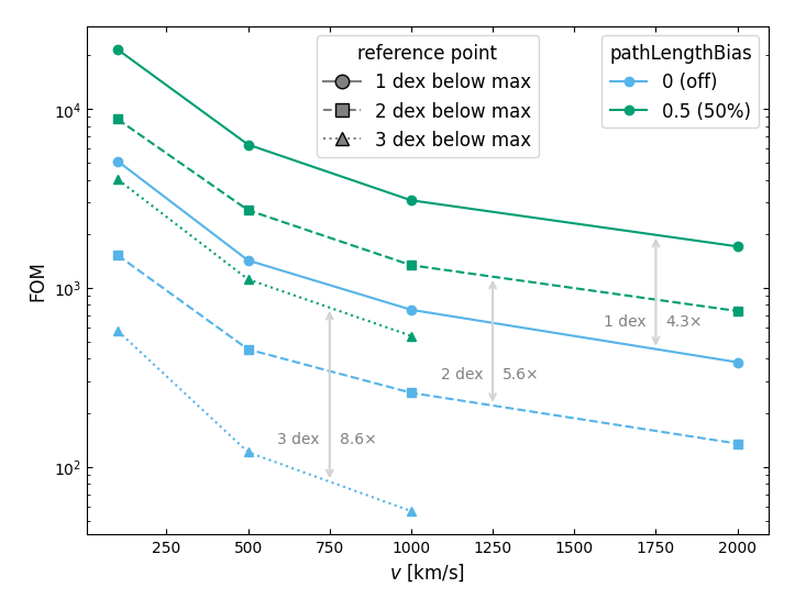
The figure above shows the converged FOM as a function of outflow velocity, evaluated at each of those three reference wavelengths, for disabled PLS (light blue) and for PLS with the default bias value of 0.5 (green). The light gray arrows mark the average ratio between the two, averaged over the four simulated velocities. PLS is clearly beneficial at every velocity tested, from 100 up to 2000 km/s: the FOM improvement stays remarkably flat across the tested range. Interestingly, the average improvement grows from a factor of about 4.3 at 1 dex below peak, to about 5.6 at 2 dex, to about 8.6 at 3 dex. This is what one would expect given that PLS was designed to ease access to low-probability regions.
This test uses a deliberately simple model with a very smooth velocity distribution. We therefore ran a similar test for a model with 300 randomly moving pockets of material. The optical depth along a full coordinate axis is between 11 and 15. The individual pockets have velocities ranging from 380 km/s to 3160 km/s with a mean of 2000 km/s, in random directions. This test confirms the overall trend seen with the smooth model: the simulations with enabled PLS show a FOM improvement by a factor of 4 or more (detailed results not shown here).
These results should not be over-generalized. Specifically, the medium parameters used in these tests are well within the previously established comfort zone of moderate optical depth and non-negligible absorption (see The comfort zone, High optical depth, High albedo). The addition of kinematics to the mix may influence the boundaries of the comfort zone in unexpected ways.
In summary, it seems that the PLS technique works well for simulations that include kinematics, as long as the material parameters stay within the comfort zone.
To check whether the encouraging kinematics result above carries over to X-ray radiative transfer, we repeat the exercise for a static, ring-shaped torus of neutral atomic gas (XRayAtomicGasMix, which models photo-absorption, fluorescence, and bound-electron scattering) around a central X-ray point source with a cutoff power-law spectrum. The setup follows the RXTORUS benchmark configuration described in Vander Meulen et al. 2023 [ADS], section 4.2.2; see X-ray reprocessing by smooth torus on this web site for a full description and a comparison against the REFLEX code. We use an equatorial column density of \(N_\mathrm{H}=10^{23}~\mathrm{cm}^{-2}\), viewed along an obscured sightline at an inclination of 75°, and compare PLS switched off against PLS with bias 0.5 (the default), at photon packet counts up to \(10^8\).
An X-ray spectrum like this one is not a single smooth feature the way the kinematics test above was: the scientifically interesting part of the reprocessed signal consists of several very narrow fluorescence lines sitting on top of a smooth continuum. To capture both aspects, we evaluate the FOM at five reference points in the energy range below 1 keV: two in the line-free continuum, and the centres of the three most prominent fluorescence lines in this range, which turn out to be the Kα lines of nitrogen, oxygen, and neon.
We could not use similar reference points above 1 keV. SKIRT's recorded noise statistics are based on the total detected signal, including light that reaches the instrument without ever interacting with the torus. Above roughly 1 keV the torus becomes increasingly transparent, so this directly transmitted light increasingly dominates the detected total and makes the recorded statistics look artificially good – they no longer reflect the noise on the scattered and re-emitted (fluorescence) signal that is actually of interest here. Below 1 keV, the torus absorbs virtually all of the direct light, so this problem does not arise and the recorded statistics are meaningful.
| Reference point | Energy (keV) | FOM ratio (bias 0.5 / off) |
|---|---|---|
| Continuum | 0.35 | 0.56 |
| N Kα line | 0.39 | 0.57 |
| O Kα line | 0.53 | 0.60 |
| Continuum | 0.75 | 0.58 |
| Ne Kα line | 0.85 | 0.67 |
At every one of these five points, enabling PLS reduces the figure of merit to at best two thirds of its value with PLS switched off, both in the continuum and on the fluorescence lines. Unlike the kinematics case above, PLS is therefore not beneficial for this X-ray torus configuration, even though its column density sits within the established comfort zone. However, in this medium the cross section varies significantly with wavelength. At the same time, many photon packets experience strong wavelength updates along their path as a result of Compton scattering and fluorescence transitions (which are implemented as scattering). Most likely this causes the poor PLS performance.
In conclusion, for this type of medium, PLS should be left switched off.
Lyman-alpha and similar resonant scattering regimes often show optical depths of 1000 and higher at the center of the resonant line. Furthermore, in the absence of other media, there is no absorption at all – just scattering. As discussed in the previous sections (High optical depth and High albedo), this is a nightmare scenario for the PLS technique.
Moreover, because of the very short free path lengths between interactions, resonant scattering is best simulated with a non-forced-scattering photon cycle, for which PLS is not implemented anyway (see Non-forced-scattering photon cycle).
The SKIRT time instruments record the time-lag response to a pulse in the source luminosity. To study the behavior of PLS for such instruments, we again use the slab configuration described in The comfort zone, now equipped with a LightCurveInstrument at the same observer position. We set the transverse optical depth to 5.
|
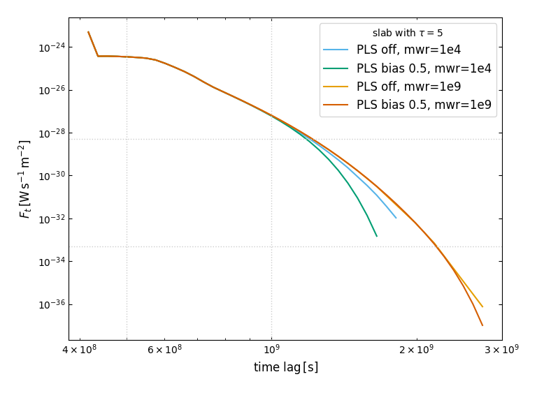
The above figure shows the light curve calculated in four different ways: without and with PLS (default bias), and minimum weight reduction set to the default value of 1e4 or boosted to 1e9. All curves are converged (launching more packets does not visibly change the curve, and the R and VOV metrics have a value below 0.1). Remarkably, the tails of these light curves differ quite significantly.
The minWeightReduction property of PhotonPacketOptions terminates a photon packet as soon as its weight drops below its original luminosity divided by this property's value; a larger value thus means a harder-to-reach cutoff. In this slab configuration, reaching a large time lag requires many consecutive scattering events, each of which multiplies the packet's weight by the local albedo. With the default value of 1e4, packets that have scattered many times are terminated well before they can contribute to the tail of the light curve, artificially truncating it. Raising the value to 1e9 lets packets survive far more scattering events, so their contribution to the late-time bins is retained and the reliable range of the light curve extends much further.
PLS makes this truncation worse. As described in Forced-scattering photon cycle, it applies an additional multiplicative bias weight at every scattering event, on top of the albedo factor. This extra weight reduction means a PLS-enabled packet reaches the minWeightReduction cutoff – and gets aborted – after fewer scattering events than an otherwise identical packet without PLS. Since reaching a given time lag requires a minimum number of scatterings, this systematically removes long-lived, late-arriving packets from the estimate, which is why the PLS-enabled curves in the figure cut off earlier than their PLS-off counterparts at the default threshold, and why the gap narrows once the threshold is raised to 1e9.
With minWeightReduction=1e4, the light curves are in agreement until around 5 dex below the peak, while the curves with minWeightReduction=1e9 remain meaningful until about 10 dex below peak (see the horizontal reference lines).
| Time lag (s) | FOM ratio (bias 0.5 / off) |
|---|---|
| 5e8 | 4.0 |
| 1e9 | 10.6 |
The two time lag points in this table are marked by the vertical reference lines in the figure. At both points, the light curves have not yet visibly diverged (they sit well above the 5 dex line discussed above). PLS delivers a significant FOM improvement by a factor of 4 to 10 in this "reliable" time lag range, independent of the minWeightReduction value.
In summary, PLS remains genuinely useful for this type of time-resolved instrument, delivering a substantial FOM improvement in the well-converged part of the light curve. However, care must be taken to raise minWeightReduction well above its default value when the low-flux, late-time tail of the light curve is of interest, since the default setting prematurely terminates exactly the long-lived packets needed to populate that region – an effect that PLS aggravates but does not cause.
When enabling PLS in a simulation that previously was run without PLS, the simulation will run faster. However, the number of photon packets must be increased to obtain the same output quality as before. This is because the stretched photon packet paths experience fewer interactions and thus spin off fewer peel-off packets to the instruments. Consequently, when making this change, one needs to perform a new convergence study (see Discretization and numerical convergence).
When in doubt, a FOM comparison (see The figure of merit and other sections above) is the only proper tool to determine whether the PLS technique is beneficial for a given type of simulation.
There is no theoretical reason for expecting improved PLS performance for values of the bias parameter \(\xi\) other than 0 and 0.5. The parameter controls the fraction of path segments for which a "stretched" interaction point is sampled. In simulation regimes where PLS does not perform well, other \(\xi\) values will simply adjust the level of bad performance. In cases where PLS does benefit the FOM, \(\xi\) values below 0.5 will lower the benefit, while \(\xi\) values above 0.5 will cause larger bias factors, resulting in higher noise levels (see Forced-scattering photon cycle). Without carrying out an in-depth study, various spot checks (not shown here) seem to confirm this reasoning.
Consequently, users should configure \(\xi=0\) to disable PLS and \(\xi=0.5\) to enable it.
SKIRT gathers the statistics information used to calculate the R and FOM metrics (see The figure of merit) while photon packets are being detected by the instruments. If a simulation performs multiple iterations to calculate self-consistent results, only the very last iteration sends peel-off photon packets to the instruments. Furthermore, no statistics are gathered on the radiation field calculated during the iteration process. The statistics thus just measure the noise originating in the last iteration; they do not provide information on the quality or level of convergence of the iterative calculation.
Similarly, in a simulation with secondary emission, the statistics do not measure the quality of the radiation field calculated during primary emission and used to determine secondary emission characteristics. Also, the statistics apply to the total detected flux. The R and FOM metrics thus cannot be obtained for primary and secondary components separately, except in spectral ranges where one component strongly dominates the other.
Explicit absorption (EA) is an alternative formulation of the photon life cycle introduced by Baes et al. (2022), exposed in SKIRT through the explicitAbsorption property of PhotonPacketOptions. Rather than sampling from the extinction optical depth along a photon packet's path, EA samples the packet's next interaction location from the scattering optical depth alone and applies absorption separately, as an independent weight factor accumulated along the path. Because this factor is decoupled from the (necessarily non-negative) scattering cross section, it can represent a genuine energy gain rather than a loss, supporting stimulated emission that may exceed the absorption in some (or all) cells along the path.
The PLS results discussed in the previous sections were performed with EA disabled. Here we offer some results related to EA based on spot checks rather than an in-depth study:
There seems to be no reason to recommend enabling EA other than, evidently, for media with stimulated emission.
| Simulation regime | Example | explicitAbsorption | forceScattering | pathLengthBias |
|---|---|---|---|---|
| balanced albedo, no extreme optical depth | dust in galaxies (UV-submm) | false | true | 0.5 |
| . the above with moving media | . | false | true | 0.5 |
| extreme optical depth | depends on geometry | false | true | 0 |
| scattering-dominated, no dispersion (*) | Thomson electrons | false | false | 0 |
| scattering dispersion (*) | Compton electrons; XRay gas | false | true | 0 |
| resonant scattering | Lyman-alpha line | false | false | 0 |
| stimulated emission | NonLTE gas lines | true | true | 0 |
(*) Scattering dispersion: scattering events update the photon wavelength (elastic scattering, fluorescence)