 |
The SKIRT project
advanced radiative transfer for astrophysics
|
|
The SKIRT project
advanced radiative transfer for astrophysics
|
This section describes how to evaluate the numerical accuracy of a SKIRT simulation, enabling reliable and scientifically robust results.
By the nature of numerical methods, SKIRT discretizes the physical quantities defining a simulated model into distinct resolution elements such as spatial cells, wavelength bins, and photon packets. Various parameters in the configuration ski file control the level of discretization. Generally speaking, a finer-grained resolution improves the approximation to the continuous variables and thus the simulation results, while also increasing the computational costs. To find a acceptable balance, and to ensure meaningful results, it is essential to perform numerical convergence tests.
The first section below describes the generic procedure for testing numerical convergence. Subsequent sections consider the following categories of physical quantities and corresponding discretization mechanisms:
For the vast majority of SKIRT simulations, the correct result is not known a priori - usually that's why we perform the simulations to begin with. We therefore need mechanisms that enhance our confidence in the simulated observables. SKIRT has been benchmarked, tested and used extensively, so we can be fairly confident in this area.
The discussion here, however, focuses on numerical issues, and specifically the effects of discretization. The SKIRT user is responsible for setting the parameters in the configuration ski file that control the level of discretization of the various model properties (spatial and spectral distributions) and simulation algorithms (photon packets). But how to find the parameter values that produce a meaningful result using an acceptable amount of compute resources?
A good starting point can often be found in papers where authors describe their use of SKIRT for applications similar to yours (see Publications Gallery). Likewise, the examples and guidelines offered in the SKIRT user guide form an important body of information (see User Guide). Still, the optimal values depend on the specific properties of the model and on the observables being simulated. It is therefore always necessary to perform further tests.
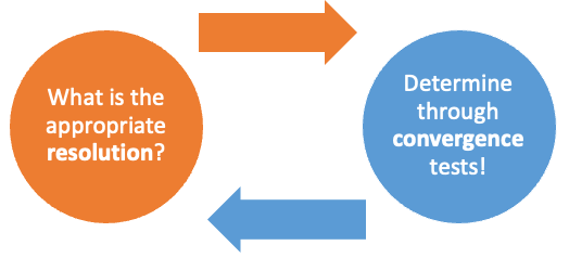
The overall idea is to refine the discretization resolution until the relevant simulated observables are converged, i.e. the observables no longer change significantly between resolution steps. The procedure can be summarized as follows:
In some specific cases you can pinpoint the proper parameter values for a simulation with a high degree of confidence based on experience or external guidance. Most often though, you need to verify convergence through the above procedure for each of the discretization mechanisms employed by the SKIRT simulations in your study. To complicate matters even more, these tests are interdependent. For example, a finer spatial or spectral grid requires a larger number of photon packets to propertly sample the smaller cells or bins. Or, vice versa, for a constant number of photon packets, higher resolution spatial or spectral grids yield increased statistical noise per cell/bin. So, where to start?
There is no "optimal" ordering of convergence tests. One approach is to alternate between the various discretization types. First establish convergence for all discretization types towards significantly relaxed observable criteria. This offers insights in how the simulation responds to parameter value changes, requiring limited compute resources because of the relaxed target criteria. Then tighten the observable criteria and again establish convergence for all discretization types.
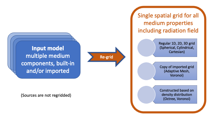
In a SKIRT simulation, the spatial distributions of all transfer medium properties are discretized on a single internal spatial grid. This includes input model properties such as the local density for each medium component as well as calculated properties such as the radiation field. Property values are considered to be uniform within each cell of the spatial grid. To properly resolve the medium, small cells must be placed in regions where input model properties and/or calculated properties vary rapidly. A higher resolution grid will generally enable more accurate simulation results, while significantly increasing computational costs in terms of both memory usage and runtime.
Because all medium properties in the simulation's input model are discretized on the same spatial grid, (re-)gridding is necessary during setup in most cases. This mechanism allows SKIRT to handle a wide range of input model types (even in the same simulation), including mathematically-defined built-in density profiles and distributions interpolated from a set of smoothed particles or tabulated on structured or unstructured grids. In all cases, SKIRT samples the input model at a (user-configurable) number of random locations within each cell of the internal spatial grid to determine the average property values.
As an aside, note that information about primary sources is not stored on the internal spatial grid. Locations for emitting photon packets are sampled straight from the input model definition while the simulation progresses, without any regridding. On the other hand, secondary sources are defined on the internal spatial grid because their properties are calculated on that grid during the simulation. Photon locations for secondary emission are thus sampled on the internal spatial grid.
SKIRT offers a wealth of spatial grid types, ranging from regular grids with spherical or cylindrical symmetries to structured or unstructured adaptive grids. Selecting and configuring an appropriate grid for a given simulation is an essential but often nontrivial task.
For more information, see:
Wavelength plays an important role in SKIRT simulations because interactions between radiation and matter are usually wavelength-dependent, and the wavelength of an interacting photon may change along its path. Therefore, SKIRT offers an advanced and thus fairly involved treatment of wavelengths and spectral discretization.
Each photon packet has a wavelength property that can take on any floating point value, i.e. it is not discretized. A photon packet's wavelength can therefore be considered to be "exact", and it can be updated with "exact" precision whenever an interaction requires this.
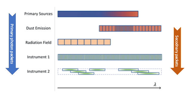
Most source spectra employed by SKIRT are tabulated on some wavelength grid. Possibilities include a built-in SED or SED family, an input file provided by the user, or for secondary emission, a table calculated by a previous phase in the simulation. In all cases, during emission, a wavelength is sampled straight from the tabulated source spectrum using log-log interpolation. Each source spectrum can use its own specific wavelength grid and there is no regridding.
On the other hand, a wavelength-dependent quantity calculated and stored during the simulation must be discretized on some wavelength grid with a finite number of bins. Because each simulation has different requirements and memory usage limitations, this wavelength grid must be configured by the user. Specifically, SKIRT employs a user-configured wavelength grid for storing the radiation field in simulations that require it, usually to enable secondary emission calculations. Because the radiation field is stored for every spatial cell, the number of bins in the spectral grid must be carefully managed to avoid excessive memory usage. On the other hand, the number of bins should be sufficiently large to properly resolve the spectral signature of the radiation field, enabling accurate calculation of secondary emission spectra.
Furthermore, each instrument in the simulation must be configured with a wavelength grid to store the fluxes being recorded. These wavelength grids should be fine-tuned to fit the needs of the use case while keeping an eye on the required computational resources. Increasing the spectral resolution will deteriorate the signal-to noise ratio in individual wavelength bins unless the number of photon packets in the simulation is increased. Also, because IFU data cubes can be large, it is sometimes useful to assign a lower-resolution grid to a FrameInstrument in combination with a higher-resolution grid for an SEDInstrument in the same sight line. This boosts the signal-to noise ratio in the data cube pixels while also limiting memory usage.
One last type of spectral discretization is used for calculating secondary emission in each spatial cell. For example, calculating the emission spectrum of a dust grain population embedded in a given radiation field requires a fairly high-resolution wavelength grid. Fortunately, this grid is used on the fly while processing secondary emission for a given cell and thus does not contribute much to memory usage.
For more information, see:
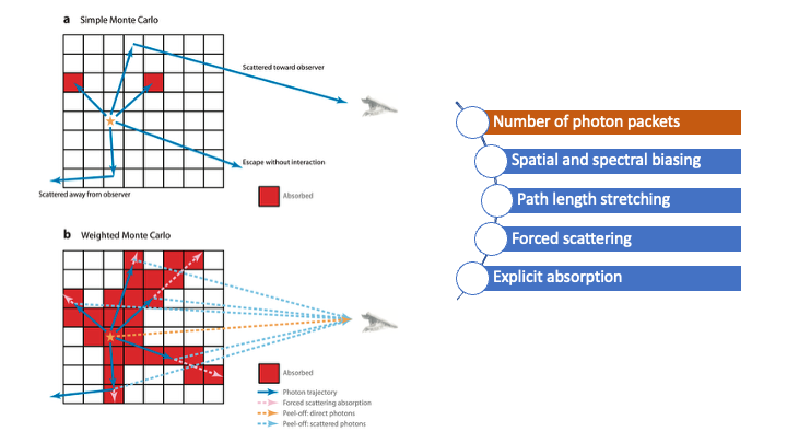
SKIRT represents the flow of radiation through the spatial domain by a large number of photon packets. The origin and interactions of each photon packet are determined probabilistically and its contribution to the simulated observables is recorded. In the limit of an infinite number of packets, this produces the intended results. With a more achievable finite number of packets, the results inevitably show Monte Carlo noise.
It is the user's responsibility to choose a number of photon packets so that (a) all relevant regions in the spatial domain are properly sampled by the random paths, and (b) the Monte Carlo noise is at an acceptable level for the key simulated observables. This is best achieved by performing convergence tests as described earlier in this topic.
In addition, SKIRT offers some contol over the photon packet cycle employed during this process. These parameters can usually be left to their default values, but some simulations can benefit from adjustments.
For more information, see:
SKIRT implements many photon-material interactions. In some cases, the corresponding wavelength-dependent behavior can be easily modeled mathematically and is thus hardwired in code. More often, specific material properties are built into SKIRT as tabulated resources. The user does not have any control over the resolution of these tables nor over the interpolation mechanisms used to extract information from them.
One notable exception is the treatment of dust grain size distributions in simulations with secondary dust emission. The dust emission spectrum depends on the grain size, so the dust grain population must be discretized into a number of size bins. In this case, the user can configure the number of these bins.
For more information, see: