This page offers an overview of the various types of probes offered by SKIRT and their capabilities. The discussion is organized as follows:

Types of probes

Generally speaking, SKIRT generates two types of output from a simulation: instruments produce synthetic observations of the simulated model, while probes sample numerical or physical quantities internal to the simulated model. Probes thus provide relevant diagnostics on the simulation setup and offer an opportunity to investigate properties of the simulated model that could never be directly observed from the outside, such as for example the radiation field.

A simulation can be configured with any number of probes and can include multiple probes of the same type. This can be useful to probe the same quantity in various ways, perhaps at different positions or wavelengths or at different stages during the simulation. In fact, SKIRT includes dozens of probe types and many of those have several user options that determine the precise operation of the probe.

A probe is an instance of one of the Probe subclasses. At the highest level, the Probe class hierarchy is split in three categories as illustrated in the diagram below.

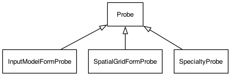
The input model probes (InputModelFormProbe subclasses) probe quantities defined by the input model, provided the relevant data is retained in memory by the simulation. Examples include the luminosity of primary sources and the mass density distribution of media. In the current implementation, these probes work only for imported sources and media. Because they operate directly on the original, imported data structures, there are no re-gridding effects in the output generated by these probes.

The internal spatial grid probes (SpatialGridFormProbe subclasses) probe quantities discretized over the spatial grid that is used in the simulation to perform radiative transfer. This includes quantities directly derived from the input model and re-gridded to the internal grid during setup, such as the mass density, and quantities calculated during the simulation, such as the radiation field. These probes work regardless of whether the input model was imported or defined using built-in geometries.

The third category contains specialty probes (SpecialtyProbe subclasses) that do not fit in another category for one reason or another. This includes probes tracking numerical aspects of the simulation, such as the number of photon packets being launched, or probes that output statistics on the quality of the internal spatial grid.

Forms

The probes in the first two categories (input model and internal grid) all share a common mechanism to define how a given quantity must be probed. The goal is to allow combining two orthogonal concepts in an arbitrary fashion. The quantity being probed is specified by the probe (a Probe subclass), while the manner in which this quantity is being probed is specified by a form (a Form subclass). The table below lists the available Form subclasses; for more information refer to the respective class documentation.

Form subclass	File format	Output
PlanarCutsForm	FITS	Cut along a specified plane parallel to one of the coordinate planes
ParallelProjectionForm	FITS	Parallel projection towards a specified sight line (inclination, azimuth)
AllSkyProjectionForm	FITS	All-sky projection towards a specified position, usually inside the model
LinearCutForm	Column text	Rows for positions along a specified line segment
MeridionalCutForm	Column text	Rows for positions along a specified meridional arc
AtPositionsForm	Column text	Row for each position listed in an input file
- Only applicable to internal spatial grid probes:
DefaultCutsForm	FITS	Default cuts along the coordinate planes
PerCellForm	Column text	Row for each internal grid cell

For input model and internal grid probes, each probe must thus be configured with an associated form. By associating multiple probes of the same type with a form with different properties or a different type of form, one can easily probe a given quantity (e.g., dust mass density) in various ways (e.g., cuts along different planes or projections from different sight lines).

For planar cuts, the model or grid is sampled at the center of each output pixel. Similarly, for planar projections, a ray is sent through the model or grid for each output pixel center, calculating the projection by accumulating information along that ray. Consequently, the probed output ignores small features in the model that intersect/project on the pixel but do not overlap the pixel center. To improve accuracy, decrease the pixel size by increasing the number of pixels along each axis.

Most of the forms can be associated with any probe types, except that some forms do not work with the input model probes because they require the internal spatial grid. This includes the PerCellForm, for obvious reasons, and the DefaultCutsForm, because it requires the extent of the simulation's spatial grid.

The PerCellForm and 3D distributions

The output of any spatial grid probe equipped with the PerCellForm can be used to extract a full 3D distribution or to construct a volumetric plot of the quantity being probed. To achieve this, the simulation configuration should also include an instance of the SpatialCellPropertiesProbe. This specialty probe outputs information for each spatial grid cell, including the x,y,z coordinates of the cell center and the cell volume, in the same order as the PerCellForm output files. This allows associating spatial information with the probed quantity

For example, when using an octree grid, each grid cell has the same form factor as the complete spatial domain (a cube or a cuboid). Given the center and volume of a cell it is easy to reconstruct the cell corner coordinates. One can then determine the containing cell for an arbitrary point in the spatial domain by searching through all the cells (possibly optimized through a search tree). For other types of grids the procedure would be similar.

Input model probes

The table below lists the available input model probes.

Probe subclass	# values	Aggregation	Configuration options
- Sources:
ImportedSourceLuminosityProbe	$N_{λ}$	System	wavelengthGrid, convolve
ImportedSourceDensityProbe	1	System	massType
ImportedSourceMetallicityProbe	1	System	weight, wavelength
ImportedSourceAgeProbe	1	System	weight, wavelength
ImportedSourceVelocityProbe	3	System	weight, wavelength
- Media:
ImportedMediumDensityProbe	1	Component
ImportedMediumMetallicityProbe	1	Component
ImportedMediumTemperatureProbe	1	Component
ImportedMediumVelocityProbe	3	Component

The second column lists the number of values for each quantity sample. The luminosity probe outputs a value for each bin in the specified wavelength grid; other than that, scalar quantities have a single value and vector quantities have three values, one for each vector component.

The third column lists the aggregation mechanism. The source probes combine information from all sources in the simulation. Therefore, they work only if all sources in the model are imported and offer the required properties. For example, the metallicity probe requires all sources to be imported and include a metallicity column as part of the parameters for the associated SED family. In contrast, the medium probes produce separate output for each individual medium component. They simply skip any components that are not imported or do not offer the required properties.

The last column lists the options to configure these probes, other than the probe name and the form associated with the probe.

The luminosity probe obviously requires a wavelength grid (for more information on wavelength grids, see Wavelength grids overview). If the convolve option is false, the specific luminosity is sampled at the characteristic wavelength of each bin. If the convolve property is true, the specific luminosity is averaged over the width of each wavelength bin (for disjoint wavelength grids) or convolved over each broadband transmission curve (for band wavelength bins). When associated with a ParallelProjectionForm, this probe can thus produce transparent noise-free narrowband or broadband images of the imported sources.

The source density probe outputs the initial or current mass density accumulated over all imported sources. Most single-stellar-population (SSP) SED families require the initial mass of the stellar population as an import parameter. On the other hand, stellar mass maps should be based on the current population mass. Therefore, this probe offers the massType option. When set to InitialMass, the probe will use the initial mass as a suboptimal solution. However, assuming that the current mass can be obtained when preparing SKIRT's input data, a better solution is to provide it as a separate, additional column to the import process, enable the importCurrentMass option for the ImportedSource component(s), and set the massType option for the probe to CurrentMass. Now the probe will use the separately imported current mass.

The source metallicity, age and velocity probes handle averaged quantities as it is not meaningful to accumulate them over multiple sources. The weight option determines how the quantity is averaged: using the InitialMass, using the CurrentMass (see previous paragraph), or using the specific Luminosity at the wavelength specified in the wavelength option.

The medium probes do not need any of these options because the quantities being handled do not depend on wavelength and components are handled indvidually. There is, however, a caveat with respect to the averaging scheme for dust media represented as particles. See the documentation of the respective classes.

Input model probes are always executed at the end of the simulation setup phase. There is no reason to delay this any further because the quantities being handled never change during the simulation.

Internal spatial grid probes

The table below lists the available internal spatial grid probes.

Probe subclass	# values	Aggregation	Probe after	Configuration options
DensityProbe	1	Fragment, Component, Type	Setup, Run, Primary, Secondary
OpacityProbe	1	Fragment, Component, Type, System	Setup, Run, Primary, Secondary	wavelength
TemperatureProbe	1	Fragment, Component, Type	Setup, Run, Primary, Secondary
MetallicityProbe	1	Component	Setup, Run, Primary, Secondary
VelocityProbe	3	System	Setup
MagneticFieldProbe	3	System	Setup
RadiationFieldProbe	$N_{r f}$	System	Run, Primary, Secondary	writeWavelengthGrid
SecondaryDustLuminosityProbe	$N_{ℓ}$	Type	Run, Secondary
SecondaryLineLuminosityProbe	$N_{ℓ}$	Component	Run, Secondary
CustomStateProbe	$N_{c s}$	Component	Setup, Run, Primary, Secondary	indices

The second column lists the number of values for each quantity sample. Scalar quantities have a single value and vector quantities have three values, one for each vector component. The radiation field probe outputs a value for each bin in the radiation field wavelength grid configured for the simulation. The last two probes in the table are briefly described in subsections below.

The third column lists the supported aggregation mechanisms. Depending on the probe type, the options include output per individual medium component, per type of medium (dust, electrons, gas), and/or for the complete medium system. Quantities such as density cannot be aggregated across medium types because, for example, dust is characterized by mass density and gas by number density. On the other hand, the simulation stores just a single bulk velocity field for all media in the system (see Sampling properties). Some probes offers a specialty aggregation option to output information for each fragment in a dust mix decorated by the FragmentDustMixDecorator. Refer to the corresponding probe class documentation for more information.

The fourth column indicates the options that specify when the probe will be performed during the simulation. Possibilities include at the end of the setup phase, at the very end of the simulation run, and after each primary or secondary iteration. Most probes are performed by default after setup, reflecting the initial (and often immutable) state of the medium system. However, quantities such as the radiation field or the dust temperature can be meaningfully probed after at least some part of the simulation has completed, so these probes are performed by default at the end of the simulation. Some simulations self-consistently adjust the medium state, for example to reflect radiative dust destruction or to calculate energy level populations in atoms or molecules. In those cases, a probe may be configured to execute after each primary or secondary iteration or at the very end of the simulation.

Probes with multiple aggregation or probe-after possibilities offer the aggregation or probeAfter configuration options, respectively. The last column in the table lists any options in addition to these and to the probe name and form associated with the probe.

The dust luminosity probe

The SecondaryDustLuminosityProbe probes the dust luminosity aggregated over all dust media as a function of wavelength, ignoring any kinematic effects, as discretized on the spatial grid of the simulation. By combining with an appropriate probe form, one can, for example, obtain the dust luminosity spectrum for each spatial cell or construct noise-free images of the transparent dust surface brightness (i.e. ignoring the effects of scattering or absorption on the secondary radiation).

The line luminosity probe

The SecondaryLineLuminosityProbe similarly probes the line luminosities of secondary sources as discretized on the spatial grid of the simulation, ignoring any kinematic effects. It produces a separate output file for each medium component with an associated material mix that exhibits secondary line emission. Examples include the SpinFlipHydrogenGasMix and the NonLTELineGasMix. For more information, see the documentation for the SecondaryLineLuminosityProbe and MaterialMix classes.

The custom state probe

The CustomStateProbe is intended for advanced users and developers. It probes the custom medium state quantities for medium components configured with a material mix that requests such variables. Examples include the dust fragment weights used by the FragmentDustMixDecorator, the neutral and atomic hydrogen fractions required by the SpinFlipHydrogenGasMix, and the energy level population densities used by the NonLTELineGasMix. For more information, see the documentation for the CustomStateProbe, MediumState, and MaterialMix classes.

Specialty probes

This category includes probes that do not fit in the categories discussed above because they probe aspects of the simulation that are not given in the input model or stored on the internal grid, or because they generate output that does not fit the form paradigm, or both.

The table below lists the available specialty probes with a brief description. For more information, refer to the respective class documentation.

Probe subclass	File format	Output
- Spatial grid statistics:
ConvergenceInfoProbe	Free-form text	Statistics on the spatial grid for each material type
ConvergenceCutsProbe	FITS	Coordinate-plane cuts through both the input and grid-discretized media density
SpatialCellPropertiesProbe	Column text	Coordinates, volume, optical depth, and densities for each spatial cell
SpatialGridPlotProbe	Data text	Info that allows plotting the structure of the spatial grid with PTS
TreeSpatialGridTopologyProbe	Data text	Topology of the tree spatial grid that can be loaded by FileTreeSpatialGrid
- Material properties:
OpticalMaterialPropertiesProbe	Column text	Cross sections etc. for the material mixes in the simulation
DustGrainPopulationsProbe	Column text	Statistics on the dust grain populations in the simulation
DustGrainSizeDistributionProbe	Column text	Size distributions of dust grain populations in the simulation
DustEmissivityProbe	Column text	Emissivity spectra for the dust mixes in the simulation
- Source statistics:
LaunchedPacketsProbe	Column text	Number of photon packets launched from sources per wavelength bin
LuminosityProbe	Column text	Primary source luminosities per wavelength bin
- Wavelength grids:
RadiationFieldWavelengthGridProbe	Column text	Wavelength, width, and borders for each radiation field wavelength bin
DustEmissionWavelengthGridProbe	Column text	Wavelength, width, and borders for each dust emission wavelength bin
InstrumentWavelengthGridProbe	Column text	Wavelength, width, and borders for each instrument wavelength bin
- Other:
SpatialGridSourceDensityProbe	Column text	Discretization of geometric source luminosity on the spatial grid
DustAbsorptionPerCellProbe	Column text	Luminosity absorbed by dust for each cell in the spatial grid