 |
The SKIRT project
advanced radiative transfer for astrophysics
|
|
The SKIRT project
advanced radiative transfer for astrophysics
|
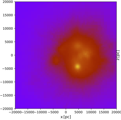
Illustration above: dust temperature map along one of the coordinate planes for the SPH-simulated galaxy used in this tutorial.
In this tutorial you will use SKIRT to study the dust in a galaxy model produced by the EAGLE cosmological simulations (http://icc.dur.ac.uk/Eagle ; http://eagle.strw.leidenuniv.nl). The EAGLE simulation code, an adjusted version of Gadget-3 (http://wwwmpa.mpa-garching.mpg.de/gadget), includes a gravitational solver for dark and baryonic matter and uses smoothed particles to implement the hydrodynamical evolution of the gas (SPH = smoothed particle hydrodynamics). The simulation results are stored in consecutive snaphots as time progresses. For this tutorial, you will use data for a single galaxy extracted from a snapshot of a pre-production EAGLE test run. Two data files are provided, respectively listing stellar particles, representing the radiation sources, and gas particles, from which a dust distribution can be derived.
This tutorial assumes that you have completed the introductory SKIRT tutorial Monochromatic simulation of a dusty disk galaxy, or that you have otherwise acquired the working knowledge introduced there. At the very least, before starting this tutorial, you should have installed the SKIRT code, and preferably also PTS and a FITS file viewer such as DS9 (see Installation Guide).
To complete this tutorial, you need the files containing the data extracted from the EAGLE snapshot in a format appropriate for importing into SKIRT. Download the files eagle_stars.txt and eagle_gas.txt using the links provided in the table below and put them into your local working directory.
| Stellar particles | eagle_stars.txt |
|---|---|
| Gas particles | eagle_gas.txt |
In a terminal window, with your local working directory as the current directory, start SKIRT without any command line arguments. SKIRT responds with a welcome message and starts an interactive session in the terminal window, during which it will prompt you for all the information describing a particular simulation:
   Welcome to SKIRT v___
   Running on ___ for ___
   Interactively constructing a simulation...
 ? Enter the name of the ski file to be created: PanEagle
The first question is for the filename of the ski file. For this tutorial, enter "PanEagle".
In this and subsequent tutorials, we skip the questions for which there is only one possible answer. The answers to these questions are provided without prompting the user, and listing them here would bring no added value.
   Possible choices for the user experience level:
      1. Basic: for beginning users (hides many options)
      2. Regular: for regular users (hides esoteric options)
      3. Expert: for expert users (hides no options)
 ? Enter one of these numbers [1,3] (2): 1
As discussed in a previous tutorial (see Experience level), the Q&A session can be tailored to the experience level of the user. For this tutorial, select the Basic level.
   Possible choices for the units system:
      1. SI units
      2. Stellar units (length in AU, distance in pc)
      3. Extragalactic units (length in pc, distance in Mpc)
 ? Enter one of these numbers [1,3] (3):
   Possible choices for the output style for wavelengths:
      1. As photon wavelength: λ
      2. As photon frequency: ν
      3. As photon energy: E
 ? Enter one of these numbers [1,3] (1):
   Possible choices for the output style for flux density and surface brightness:
      1. Neutral: λ F_λ = ν F_ν
      2. Per unit of wavelength: F_λ
      3. Per unit of frequency: F_ν
      4. Counts per unit of energy: F_E
  ? Enter one of these numbers [1,4] (3):
As discussed in a previous tutorial (see Units), SKIRT offers several output unit options. For the current tutorial, you will be modelling a galaxy, so select extragalactic units with the wavelength output style for the spectral variable and per-frequency output style for fluxes (the default options). The output files will express integrated flux density in Jy and surface brightness in MJy/sr.
   Possible choices for the overall simulation mode:
      1. No medium - oligochromatic regime (a few discrete wavelengths)
      2. Extinction only - oligochromatic regime (a few discrete wavelengths)
      3. No medium (primary sources only)
      4. Extinction only (no secondary emission)
      5. Extinction only with Lyman-alpha line transfer
      6. With secondary emission from dust
      7. With secondary emission from gas
      8. With secondary emission from dust and gas
 ? Enter one of these numbers [1,8] (4): 6
As discussed in a previous tutorial (see Simulation mode), the answer to this question determines the wavelength regime of the simulation (oligochromatic or panchromatic) and sets the overall scheme for handling media in the simulation. In this tutorial, the goal is to produce a spectral energy distribution (SED) including UV to infrared wavelengths and the effects of the emission by stochastically heated dust grains. By definition this requires a panchromatic simulation and dust emission. Select the option called "With secondary emission from dust".
? Enter the default number of photon packets launched per simulation segment [0,1e19] (1e6): 5e6
To limit the run time for this tutorial, set the number of photon packets to \(5 \times 10^6\). This number is sufficient to produce an acceptable SED for the simple galaxy model used here, but it would be insufficient to produce resolved images with an acceptable signal to noise level.
 ? Enter the shortest wavelength of photon packets launched from primary sources [1e-6 micron,1e6 micron] (0.09 micron):
 ? Enter the longest wavelength of photon packets launched from primary sources [1e-6 micron,1e6 micron] (100 micron):
For a panchromatic simulation, the source system requests the limits of the wavelength range to be considered for primary sources. For this tutorial, simply accept the suggested default values, yielding a range of \(0.09~\mu{\text{m}} <= \lambda <= 100~\mu{\text{m}}\).
   Possible choices for item #1 in the primary sources list:
      1. A primary point source
      2. A primary source with a built-in geometry
      3. A primary source imported from smoothed particle data
        ...
 ? Enter one of these numbers or zero to terminate the list [0,6] (2): 3
 ? Enter the name of the file to be imported: eagle_stars.txt
In this tutorial, the primary sources are given as a list of smoothed stellar particles in a column text file format appropriate for importing in SKIRT. Select the appropriate source component type and enter the name of your stellar particle data file, i.e. "eagle_stars.txt".
   Possible choices for the SED family for assigning spectra to the imported sources:
      1. A black body SED family
      2. A Castelli-Kurucz SED family for stellar atmospheres
      3. A Bruzual-Charlot SED family for single stellar populations
         ...
 ? Enter one of these numbers [1,9] (1): 3
   Possible choices for the assumed initial mass function:
      1. Chabrier IMF
      2. Salpeter IMF
 ? Enter one of these numbers [1,2] (1):
   Possible choices for the wavelength resolution:
      1. Low wavelength resolution (1221 points)
      2. High wavelength resolution (6900 points)
 ? Enter one of these numbers [1,2] (1):
For imported sources, each individual entity (i.e., in this case, each particle) is assigned an appropriate emission spectrum (SED) from a set of templates called an SED family. SKIRT includes some frequently-used SED families for single stellar populations (SSPs), such as those prepared and published by Bruzual & Charlot in 2003. These SED families require three parameters: the initial mass, the metallicity, and the age of the stellar population.
Select the Bruzual-Charlot SED family with the Chabrier initial mass function and the lowest wavelength resolution (both the default options). The higher wavelength resolution is relevant only when evaluating simulation results in narrow wavelength ranges.
Let us have a look at the first few lines of the "eagle_stars.txt" stellar particle file:
# Stellar particles for a simulated galaxy (pre-production EAGLE run)
# SKIRT 9 import format for a particle source with the Bruzual Charlot SED family
#
# Column 1: x-coordinate (kpc)
# Column 2: y-coordinate (kpc)
# Column 3: z-coordinate (kpc)
# Column 4: smoothing length (kpc)
# Column 5: initial mass (Msun)
# Column 6: metallicity (1)
# Column 7: age (Gyr)
#
50.14044 -39.14663 -21.36022 31.15748 1319629 0.005035158 3.761856
...
Lines starting with a hash sign (#) contain comments intended for human beings; the other lines contain information (columns of data values) for each particle. The comments are generally ignored by SKIRT with the important exception that they may contain column descriptors, as they do in this example. Specifically, the lines starting with "# Column" are recognized by SKIRT as column descriptors that convey information on the data values in the file. SKIRT recognizes and uses the units specified between parentheses. If the file contains no column descriptors, the data values must be specified in the default units as described in the documentation of the class(es) handling the import.
The first three columns in the file specify the \(x\), \(y\) and \(z\) coordinates of the particle and the fourth column is the smoothing length \(h\). The number and interpretation of the subsequent columns depends on the specified SED family. For the Bruzual-Charlot family, the remaining three columns provide the properties of the stellar population represented by each particle: its initial mass \(M_\mathrm{init}\) at \(t=0\), its metallicity \(Z\) (as a dimensionless fraction) and its age.
When asked for a second stellar component, enter zero to terminate the list.
   Possible choices for the wavelength grid for storing the radiation field:
      1. A logarithmic wavelength grid
      2. A nested logarithmic wavelength grid
      3. A linear wavelength grid
         ...
 ? Enter one of these numbers [1,7] (1): 1
 ? Enter the shortest wavelength [1e-6 micron,1e6 micron]: 0.09
 ? Enter the longest wavelength [1e-6 micron,1e6 micron]: 100
 ? Enter the number of wavelength grid points [2,2000000000] (25): 25
Primary sources assign randomly sampled wavelengths to the launched photon packets. These wavelengths can have any floating point value in the primary source range configured for the simulation (here \(0.09~\mu{\text{m}} <= \lambda <= 100~\mu{\text{m}}\)). However, it is impossible to use a similar "infinite" resolution when recording wavelength dependent information on the radiation field in each spatial cell. By necessity, this information must be stored in a finite number of wavelength bins. Because there may be many spatial cells in the simulation, the number of wavelength bins used for storing the radiation field has a substantial effect on the memory consumption of the simulation.
SKIRT offers several types of wavelength grids that can be used for discretizing a wavelength range:
For storing the radiation field in this tutorial simulation, configure a logarithmic wavelength grid with a range that matches the primary source range ( \(0.09~\mu{\text{m}} <= \lambda <= 100~\mu{\text{m}}\)) and has the default number of 25 bins.
   Possible choices for the wavelength grid for calculating the dust emission spectrum:
      1. A logarithmic wavelength grid
      2. A nested logarithmic wavelength grid
      3. A linear wavelength grid
         ...
 ? Enter one of these numbers [1,7] (1): 2
 ? Enter the shortest wavelength of the low-resolution grid [1e-6 micron,1e6 micron]: 1
 ? Enter the longest wavelength of the low-resolution grid [1e-6 micron,1e6 micron]: 1000
 ? Enter the number of wavelength grid points in the low-resolution grid [2,2000000000] (25): 75
 ? Enter the shortest wavelength of the high-resolution subgrid [1e-6 micron,1e6 micron]: 3
 ? Enter the longest wavelength of the high-resolution subgrid [1e-6 micron,1e6 micron]: 30
 ? Enter the number of wavelength grid points in the high-resolution subgrid [2,2000000000] (25): 35
Similarly, the thermal emission spectrum for the dust in each spatial cell can only be calculated at a finite number of wavelength grid points. This calculation happens on the fly, i.e. the spectrum does not need to be stored for all spatial cells at the same time. As a result, the impact of the number of wavelength grid points on memory consumption is limited, but there will still be an impact on performance.
In this tutorial simulation, you will include the effects of stochastically heated dust grains, which manifest themselves as specific spectral features at infrared wavelengths. To properly capture these features, the dust emission wavelength grid must have sufficient resolution in the relevant range.
For calculating the dust emission spectrum in this tutorial simulation, select a nested logarithmic wavelength grid ranging from 1 to 1000 \(\mu\)m, with a finer subgrid in the range from 3 to 30 \(\mu\)m. Specify 75 points in the wider grid, and 35 points in the nested grid. The points of the courser grid that happen to lie inside the finer grid range are automatically removed, so the total number of grid points will be smaller than 110.
   Possible choices for item #1 in the transfer media list:
      1. A transfer medium with a built-in geometry
      2. A transfer medium imported from smoothed particle data
         ...
 ? Enter one of these numbers [1,5] (1): 2
 ? Enter the name of the file to be imported: eagle_gas.txt
   Possible choices for the type of mass quantity to be imported:
      1. Mass (volume-integrated)
      2. Number (volume-integrated)
 ? Enter one of these numbers [1,2] (1): 1
 ? Enter the fraction of the mass to be included (or one to include all) [0,1] (1): 0.2
 ? Do you want to import a metallicity column? [yes/no] (no): yes
 ? Do you want to import a temperature column? [yes/no] (no): no
In this tutorial, the dust contents of the configured model is derived from the spatial distribution of the gas in the SPH snapshot produced by the EAGLE simulation. SKIRT estimates the dust density distribution from the gas particle data through a simple scheme: the dust density is assumed to be proportional to the density of the metallic gas. The metal fraction for each particle must be included in the imported file. The constant proportionality factor is provided as a parameter in the configuration.
Select the "imported from smoothed particle data" medium component type and enter the name of your gas particle data file, i.e. "eagle_gas.txt". Select the "mass" quantity type, set the proportionality factor to a value of 0.2, and request that SKIRT imports a metallicity column. The gas mass specified for the particle in the file will automatically be multiplied by both the constant factor and the metallicity value for the particle in the file. Finally, decline importing a temperature column. This column can be used to suppress dust in gas above a certain kinetic temperature, but this tutorial's example file does not include a temperature column.
The first lines of the "eagle_gas.txt" file are:
# Gas particles for a simulated galaxy (pre-production EAGLE run)
# SKIRT 9 import format for a medium source using M_dust = f_dust x Z x M_gas
#
# Column 1: x-coordinate (kpc)
# Column 2: y-coordinate (kpc)
# Column 3: z-coordinate (kpc)
# Column 4: smoothing length (kpc)
# Column 5: gas mass (Msun)
# Column 6: metallicity (1)
#
85.32513 101.0889 -69.36465 55.21837 2081983 2.549941e-05
...
The first three columns are the \(x\), \(y\) and \(z\) coordinates of the gas particle, the fourth column is its SPH smoothing length \(h\), the fifth column is its mass \(M_\mathrm{gas}\), and the sixth column is the metallicity \(Z\) of the gas (dimensionless fraction).
   Possible choices for the material type and properties throughout the medium:
      1. A typical interstellar dust mix (mean properties)
      2. A THEMIS (Jones et al. 2017) dust mix
      3. A Draine and Li (2007) dust mix
         ...
 ? Enter one of these numbers [1,10] (1): 2
 ? Enter the number of grain size bins for each of the silicate populations [1,2000000000] (5):
 ? Enter the number of grain size bins for each of the hydrocarbon populations [1,2000000000] (5):
SKIRT includes a large set of built-in dust grain properties and dust mixtures. A dust mixture represents a collection of a dust grains of various sizes and material types, such as for example silicate and graphite. For the purposes of calculating absorption and scattering, the optical properties of a complete dust mixture can be conveniently averaged over the various sub-populations, resulting in a single "representative grain", without loss of accuracy.
However, to calculate the thermal emission of a dust mixture embedded in a given radiation field, one needs to take the full size distribution into account. Indeed, the equilibrium temperature of the grains depends on their size as well as on their material properties. Depending on the radiation field, small grains may even be "stochastically heated", i.e. not in thermal equilibrium with their environment. In this case, it becomes necessary to compute the probability distribution of the internal grain energy to determine the emission spectrum. Stochastically heated grains emit at shorter wavelengths than if they were in equilibrium, which often substantially influences the infrared spectrum of a galaxy.
SKIRT discretizes the grain size distribution for each material type in a dust mix into a number of size bins. More bins means better accuracy. On the other hand, each bin consumes memory and processing time. In most cases, a number of size bins between 10 and 15 is an acceptable compromise.
There are several built-in "turn-key" dust mixes that require very little extra configuration. For this tutorial, select the THEMIS dust mix and leave the number of size bins for each grain type at the default value of 5, although in an actual research setting this number should be higher.
When asked for a second medium component, enter zero to terminate the list.
   Possible choices for the spatial grid:
      1. A 3D spatial grid in cylindrical coordinates
      2. A Cartesian spatial grid
      3. A tree-based spatial grid
 ? Enter one of these numbers [1,3] (3): 3
 ? Enter the start point of the box in the X direction ]-∞ pc,∞ pc[: -20 kpc
 ? Enter the end point of the box in the X direction ]-∞ pc,∞ pc[: 20 kpc
 ? Enter the start point of the box in the Y direction ]-∞ pc,∞ pc[: -20 kpc
 ? Enter the end point of the box in the Y direction ]-∞ pc,∞ pc[: 20 kpc
 ? Enter the start point of the box in the Z direction ]-∞ pc,∞ pc[: -20 kpc
 ? Enter the end point of the box in the Z direction ]-∞ pc,∞ pc[: 20 kpc
   Possible choices for the tree construction policy (configuration options):
      1. A tree grid construction policy using the medium density distribution
   Automatically selected the only choice: 1
 ? Enter the minimum level of grid refinement [0,99] (3): 3
 ? Enter the maximum level of grid refinement [0,99] (7): 7
 ? Enter the maximum fraction of dust contained in each cell [0,0.01] (1e-6): 5e-5
SKIRT discretizes the medium on a spatial grid, i.e. a collection of small cells in which properties such as density and radiation field are considered to be constant. Usually you have little a priori knowledge about a the spatial distribution imported from SPH simulation results. Due to the lack of spatial symmetries, the grid must be a full 3D grid. It is thus best to choose an adaptive grid that automatically forms smaller cells in denser regions. The grid will take some time to construct, but the simulation run will be faster and more accurate than if you would use a regular grid.
For this tutorial simulation, select a tree-based grid. The grid must enclose most of the dust in the system so its size must be adjusted to the domain of the input data. For the eagle_xxx.txt particle data files, you should specify a cube of 40 kpc in each direction, centered on the origin.
For this tutorial simulation, acceptable values for the grid refinement level are a minimum of 3 and a maximum of 7 (the default values). The maximum fraction of dust mass in each cell may be set to a value of \(5\times 10^{-5}\). For high-quality simulations, you will need to raise the maximum level to 10 or more, and the maximum fraction of dust mass should be set to a smaller (and thus more stringent) value. This will result in an octtree with more and smaller cells, increasing accuracy as well as execution time.
   Possible choices for the default instrument wavelength grid:
      1. A logarithmic wavelength grid
      2. A nested logarithmic wavelength grid
         ...
 ? Enter one of these numbers [1,8] (1): 1
 ? Enter the shortest wavelength [1e-6 micron,1e6 micron]: 0.09
 ? Enter the longest wavelength [1e-6 micron,1e6 micron]: 1000
 ? Enter the number of wavelength grid points [2,2000000000] (25): 750
Similar to the situation with recording the radiation field, instruments need to detect and store wavelength dependent flux contributions in a finite number of wavelength bins. The default instrument wavelength grid defines these bins for all instruments and for all probes that output wavelength dependent information. (When running the Q&A with a user experience level higher than Basic, it is possible to assign a different wavelength grid to each instrument or probe.)
For this tutorial, configure a logarithmic wavelength grid with a range of \(0.09~\mu{\text{m}} <= \lambda <= 1000~\mu{\text{m}}\), including both the primary and secondary source wavelength ranges, and with 750 wavelength grid points. Because you will be recording spatially integrated SEDs only for this tutorial, there is no problem with memory use even if you would specify a substantially larger number of wavelength grid points. However, maintaining an acceptable signal-to-noise ratio with the resulting higher wavelength resolution might necessitate a larger number of photon packets.
   Possible choices for item #1 in the instruments list:
      1. A distant instrument that outputs the spatially integrated flux density as an SED
      2. A distant instrument that outputs the surface brightness in every pixel as a data cube
      3. A distant instrument that outputs both the flux density (SED) and surface brightness (data cube)
 ? Enter one of these numbers or zero to terminate the list [0,3] (1): 1
 ? Enter the name for this instrument: fo
 ? Enter the distance to the system ]0 Mpc,∞ Mpc[: 10
 ? Enter the inclination angle θ of the detector [0 deg,180 deg] (0 deg): 90
 ? Enter the azimuth angle φ of the detector [-360 deg,360 deg] (0 deg): -90
 ? Do you want to record flux components separately? [yes/no] (no): yes
   Possible choices for item #2 in the instruments list:
      1. A distant instrument that outputs the spatially integrated flux density as an SED
      2. A distant instrument that outputs the surface brightness in every pixel as a data cube
      3. A distant instrument that outputs both the flux density (SED) and surface brightness (data cube)
 ? Enter one of these numbers or zero to terminate the list [0,3] (1): 1
 ? Enter the name for this instrument: eo
 ? Enter the distance to the system ]0 Mpc,∞ Mpc[: 10
 ? Enter the inclination angle θ of the detector [0 deg,180 deg] (0 deg): 90
 ? Enter the azimuth angle φ of the detector [-360 deg,360 deg] (0 deg): 180
 ? Do you want to record flux components separately? [yes/no] (no): yes
For this tutorial, configure two instruments of the type that outputs the total integrated flux as an SED. Specify two different viewpoints corresponding to face-on and edge-on sight lines, and a distance to the system of 10 Mpc. The galactic plane of the example galaxy in this tutorial is situated in the \(xz\) coordinate plane, leading to the following interesting set of angles:
| Instrument | Name | Inclination θ | Azimuth φ | Description |
|---|---|---|---|---|
| #1 | eo | 90 deg | -90 deg | edge-on |
| #2 | fo | 90 deg | 180 deg | face-on |
In an actual research setting you might lack information about the orientation of the imported galaxy, so that you would need to perform some test simulations (or other visualizations) to find out.
When asked for a third instrument, enter zero to terminate the list.
   Possible choices for item #1 in the probes list:
      1. Convergence: information on the spatial grid
      2. Convergence: cuts of the medium density along the coordinate planes
      3. Source: luminosities of primary sources
      4. Internal spatial grid: density of the medium
         ...
      8. Properties: basic info for each spatial cell
      9. Properties: data files for plotting the structure of the grid
     10. Properties: aggregate optical material properties for each medium
 ? Enter one of these numbers or zero to terminate the list [0,10] (1): 1
 ? Enter the name for this probe: cnv
 ? Enter the wavelength at which to determine the optical depth [1e-6 micron,1e6 micron] (0.55 micron):

   Possible choices for item #2 in the probes list:
         ...
      2. Convergence: cuts of the medium density along the coordinate planes
         ...
 ? Enter one of these numbers or zero to terminate the list [0,9] (1): 2
 ? Enter the name for this probe: dns

   Possible choices for item #3 in the probes list:
         ...
      6. Internal spatial grid: indicative temperature of the medium
         ...
 ? Enter one of these numbers or zero to terminate the list [0,9] (1): 6
 ? Enter the name for this probe: tmp
   Possible choices for the form describing how this quantity should be probed:
      1. Default planar cuts along the coordinate planes
      2. A text column file with values for each spatial cell
 ? Enter one of these numbers [1,2] (1): 1

   Possible choices for item #4 in the probes list:
         ...
 ? Enter one of these numbers or zero to terminate the list [0,9] (1): 0
Configure the following probes, in arbitrary order, and specify their names as follows.
| Probe type | Probe name |
|---|---|
| Convergence: information on the spatial grid | cnv |
| Convergence: cuts of the medium density along the coordinate planes | dns |
| Internal spatial grid: indicative temperature of the medium | tmp |
For the temperature probe, you can choose the "form" in which the quantity should be probed. This is so because various types of output can be produced for a given quantity (in this case the temperature). In Basic mode, there are just two options: FITS files showing a planar cut along each coordinate plane, or a text file listing the temperature for every cell in the spatial grid. In Regular mode, additional options become available, including for example parallel projection along a specified line of sight. For this tutorial, select the option to produce planar cuts along the coordinate planes.
Finally, when asked for the subsequent probe, enter zero to terminate the list.
SKIRT includes two distinct algorithms to calculate the thermal dust emission spectrum. The basic method, called "Equilibrium" emission, assumes that all dust grains are in local thermal equilibrium (LTE) with the surrounding radiation field. While this method is fast, it does not produce realistic results in many cases because the LTE assumption is often not justified for smaller dust grains. The more advanced method, called "Stochastic" or non-LTE emission, calculates a temperature probability distribution for those smaller grains instead of assuming a single equilibrium temperature. This is a lot more resource-intensive but produces much more realistic results for the near- and mid-infrared wavelengths.
With the Q&A set to the Basic user experience level (see Experience level), the configuration automatically defaults to the basic equilibrium method. Adjusting the configuration to use stochastic heating can be easily accomplished by opening the PanEagle.ski parameter file in a text editor. Locate the line that starts as follows:
<DustEmissionOptions dustEmissionType="Equilibrium" ...>
Replace "Equilibrium" by "Stochastic" (with that exact capitalization), and save the adjusted file.
After all questions have been answered, SKIRT writes out the resulting ski file and quits. Start SKIRT again, this time specifying the name of the new ski file on the command line, to actually perform the simulation. If the input data files are not in your current directory, you can specify the input directory on the SKIRT command line. For example:
skirt -i ../in PanEagle
The output files for this tutorial are similar to those already described for a previous tutorial (see Output files and Output files). Because the geometry in this simulation is truly three-dimensional (i.e. it has no axial or spherical symmetries), there are now three cuts through the dust density (one along each of the coordinate planes) rather than two. Similarly, there are now three cuts through the indicative dust temperature of the dust medium.
The instruments used in this tutorial each produce an SED: PanEagle_eo_sed.dat and PanEagle_fo_sed.dat are column text files representing the spectral energy distribution of the photon packets detected by the instruments. In addition to the wavelength column, there are several corresponding flux columns:
For this tutorial, the primary source is the set of imported stellar particles; the medium consists of the dust derived from the gas particles; and the secondary source is that same dust medium.
As always it is a good idea to open the file PanEagle_cnv_convergence.dat in a text editor and check the dust grid convergence metrics. With the spatial grid configuration recommended above for this tutorial, the convergence is not so good. The input and gridded values differ by up to 25 per cent. In an actual research setting, you would want to tweak the settings for the adaptive octree grid, creating more cells in the appropriate places, to obtain better convergence. Also, in this example, some of the imported gas particles lie outside the domain of the spatial grid. The dust derived from those particles counts towards the input dust mass, but is excluded from the gridded dust mass.
It is also instructive to compare the theoretical and gridded dust density cuts (e.g. ScatAMR_dns_dust_t_xy.fits and PanTorus_dns_dust_g_xy.fits) in an interactive FITS viewer or by plotting them using the following PTS command:
pts plot_convergence . --prefix=PanEagle --dex 4
It is quite apparent from this comparison that the octree grid indeed forms smaller cells in areas of higher dust density, but that - with the current settings - these cells are often too large to properly discretize the density distribution.
Open the temperature maps (e.g. PanEagle_tmp_dust_T_xz.fits) in an interactive FITS viewer or by plotting them using the following PTS command:
pts plot_temperature . --prefix=PanEagle
The cut through the \(xz\) coordinate plane should look similar to the figure shown at the start of this tutorial:
Consider the temperature gradient in the dust, and look up the minimum and maximum temperature values. As noted in a previous tutorial (see Output files), the indicative dust temperature shown in these maps does not correspond to a physical temperature, but rather reflects one of the many ways to obtain a representative temperature for a dust mixture.
PTS offers commands to create PDF files plotting the SEDs produced by a SKIRT simulation. By default, the SEDs for all instruments are combined on the same figure. The following command produces the plot shown below:
pts plot_seds . --prefix=PanEagle --dex=4
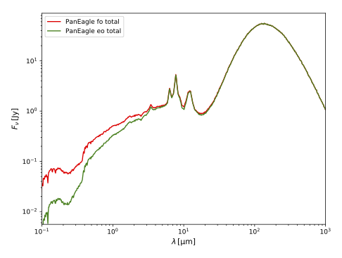
For UV, optical and near-infrared wavelengths (up to about \(8\,\mu\mathrm{m}\)) the dust extinction is substantially larger in the edge-on sight line than in the face-on sight line. This is expected since the edge-on radiation has to penetrate a lot more dust before it reaches the observer. At longer wavelengths, the interaction cross section is sufficiently small that the dust becomes almost transparent and the spectrum is essentially isotropic. Also, note the spectral features in the \(3-20\,\mu\mathrm{m}\) wavelength range, mostly resulting from the emission of stochastically heated dust grains.
The same PTS command can also plot the various flux components detected by a single instrument. For example, the following command produces the plot shown below:
pts plot_seds . --prefix=PanEagle --instr=eo --wmin=0.1 --wmax=50 --dex=3
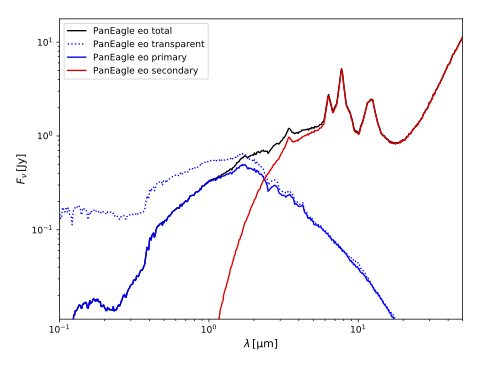
The dotted line indicates the unattenuated stellar flux, i.e. as if there were no dust in the model. It is evident that there is a dramatic amount of extinction for this sight line. The plot also nicely indicates the respective contributions of primary (stellar) and secondary (dust) emission across the wavelength range.
Congratulations, you made it to the end of this tutorial!