Configuring custom dust mixes

This advanced tutorial explores the mechanisms for configuring custom dust mixes in SKIRT. The built-in turn-key dust mixes are sufficient for many applications and should remain the preferred choice for beginning (and many advanced) users. On the other hand, the flexibility to specify a customized dust model enables many powerful applications, including:

• Investigating the effect of changing optical material properties, relative abundances, grain size distributions, and so forth on the observed extinction and emission characteristics of a given model or class of models. See section Customizing dust properties below.
• Spatially varying the properties of the dust in models imported from hydrodynamical snapshots by assigning a different type of dust (material type, grain size, etc.) to each particle or cell. See section Spatially varying the dust mix in imported models below.

Getting ready

Because this is an advanced tutorial, it assumes that:

• you have installed SKIRT and any relevant visualization tools (see Installation Guide);
• you understand the structure of ski files and know how to manually adjust them (see The SKIRT parameter file format (ski file));
• you have worked through the introductory SKIRT tutorials (e.g., Monochromatic simulation of a dusty disk galaxy and Panchromatic simulation of a dust torus);
• you have a working knowledge of interstellar dust properties, dust material types, absorption and scattering processes, grain size distributions, wavelength dependence and so forth;
• you have a basic understanding of how dust mixtures are handled in SKIRT (see Material mixes (dust, electrons, gas)).

After all of that, you are ready to take a deep dive into the world of custom SKIRT dust mixes. This tutorial offers a SKIRT parameter file for download to serve as an initial reference model. Download this file using the link provided in the table below and put it into your local working directory.

Reference model for customizing dust properties	TutorialCustomDustReference.ski

Customizing dust properties

Reference model

Rename the downloaded SKIRT parameter file to a shorter name of your liking ending with the ".ski" filename extension and run it with SKIRT. If SKIRT immediately produces a fatal error while constructing the simulation, this probably means that the ski file needs upgrading; see Upgrading SKIRT parameter files.

While the simulation is running, open the ski file in a text editor and examine its contents. It configures a basic, spherically symmetric model with a central point source surrounded by a shell of dust. The point source is assigned the typical spectrum of a fairly young stellar population. The surrounding dust is distributed as a shell with a radius of 1 pc and a shallow exponential radial density profile. The total dust mass is set to 1 solar mass. To capture as many aspects of the influence of dust properties as possible, the configuration specifies a panchromatic simulation from UV to submillimeter wavelengths taking into account stochastic heating of small grains. The built-in Zubko et al. 2004 dust mix, which you will replace in later sections by custom dust mix variations, is configured with a suffiently large number of size bins to properly resolve the grain size distributions when calculating the emission spectrum for each material type and for each representative grain size:

<ZubkoDustMix numSilicateSizes="15" numGraphiteSizes="15" numPAHSizes="10"/>

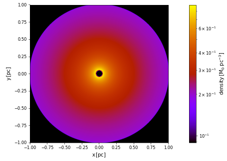
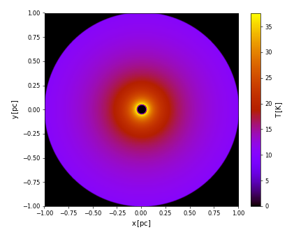
After the simulation finishes, open the text file produced by the ConvergenceInfoProbe. It should indicate a radial V-band optical depth of about 2.12. The following figures show a cut through the dust density and a cut through the indicative dust temperature, respectively generated by the ConvergenceCutsProbe and the TemperatureProbe with DefaultCutsForm.

Dust density	Indicative dust temperature

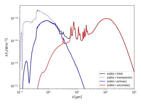
The following figure shows the SED produced by this reference configuration, separated into its stellar and dust emission components. The dashed line indicates the stellar spectrum without dust extinction.

SED for reference model with built-in Zubko et al. 2004

The OpticalMaterialPropertiesProbe ("1") outputs the aggregate optical properties of the dust mix as a function of wavelength. For convenience depending on the user's needs, the extinction properties are listed in two equivalent forms: as a cross section per hydrogen atom (in ${\mathrm{m}}^2$) and as a mass coefficient (in ${\mathrm{m}}^2{\mathrm{k}\mathrm{g}}^{-1}$). These two quantities are connected through the dust mass per hydrogen atom for the dust mix, which is listed (in $\mathrm{k}\mathrm{g}$) on the very first line of the file.

The DustGrainPopulationsProbe ("2") outputs some characteristics for each of the grain populations in the dust mix. A grain population defines a grain material type and a corresponding grain size distribution. The built-in Zubko dust mix includes four grain populations:

# ... dust mass per hydrogen atom: 1.305623577e-29 kg
...
0 Draine_Silicate     62.1543 8.115005680e-30 4.851668068e-03 ...
1 Draine_Graphite     32.8185 4.284855429e-30 2.561759915e-03 ...
2 Draine_Neutral_PAH   2.5136 3.281873294e-31 1.962113212e-04 ...
3 Draine_Ionized_PAH   2.5136 3.281873294e-31 1.962113212e-04 ...

The first column after the material type name lists the relative mass of each population in the total mix, as a percentage. The next two columns list the absolute mass in two forms: per hydrogen atom and per hydrogen mass. These numbers are provided for convenience when comparing a configured dust mix to dust models in the literature.

The DustGrainSizeDistributionProbe ("3") outputs the size distribution for each of the grain populations (in separate files). A grain size distribution is not a normalized probability distribution; the scaling of the values is taken into account when integrating over the size distribution to calculate aggregate or representative properties.

Many of these concepts will play an important role later in this tutorial.

Duplicating a built-in dust mix

Although the turn-key dust mixes built into SKIRT are hardwired in the code, they effectively use the same components as those used to configure a custom dust mix. For example, the built-in Zubko dust mix is coded as follows (see the ZubkoDustMix class):

addPopulation(new DraineSilicateGrainComposition(this), new ZubkoSilicateGrainSizeDistribution(this),
              _numSilicateSizes, GrainPopulation::NormalizationType::FactorOnSizeDistribution, 1.);
addPopulation(new DraineGraphiteGrainComposition(this), new ZubkoGraphiteGrainSizeDistribution(this),
              _numGraphiteSizes, GrainPopulation::NormalizationType::FactorOnSizeDistribution, 1.);
addPopulation(new DraineNeutralPAHGrainComposition(this), new ZubkoPAHGrainSizeDistribution(this),
              _numPAHSizes, GrainPopulation::NormalizationType::FactorOnSizeDistribution, 0.5);
addPopulation(new DraineIonizedPAHGrainComposition(this), new ZubkoPAHGrainSizeDistribution(this),
              _numPAHSizes, GrainPopulation::NormalizationType::FactorOnSizeDistribution, 0.5);

Assuming that the number of size bins for each population is configured as for the reference model above, this translates to the following equivalent ski file configuration:

<ConfigurableDustMix scatteringType="HenyeyGreenstein">
    <populations type="GrainPopulation">
        <GrainPopulation numSizes="15" normalizationType="FactorOnSizeDistribution" factorOnSizeDistribution="1">
            <composition type="GrainComposition">
                <DraineSilicateGrainComposition/>
            </composition>
            <sizeDistribution type="GrainSizeDistribution">
                <ZubkoSilicateGrainSizeDistribution/>
            </sizeDistribution>
        </GrainPopulation>
        <GrainPopulation numSizes="15" normalizationType="FactorOnSizeDistribution" factorOnSizeDistribution="1">
            <composition type="GrainComposition">
                <DraineGraphiteGrainComposition/>
            </composition>
            <sizeDistribution type="GrainSizeDistribution">
                <ZubkoGraphiteGrainSizeDistribution/>
            </sizeDistribution>
        </GrainPopulation>
        <GrainPopulation numSizes="10" normalizationType="FactorOnSizeDistribution" factorOnSizeDistribution="0.5">
            <composition type="GrainComposition">
                <DraineNeutralPAHGrainComposition/>
            </composition>
            <sizeDistribution type="GrainSizeDistribution">
                <ZubkoPAHGrainSizeDistribution/>
            </sizeDistribution>
        </GrainPopulation>
        <GrainPopulation numSizes="10" normalizationType="FactorOnSizeDistribution" factorOnSizeDistribution="0.5">
            <composition type="GrainComposition">
                <DraineIonizedPAHGrainComposition/>
            </composition>
            <sizeDistribution type="GrainSizeDistribution">
                <ZubkoPAHGrainSizeDistribution/>
            </sizeDistribution>
        </GrainPopulation>
    </populations>
</ConfigurableDustMix>

The scatteringType property of a configurable dust mix specifies the type of scattering phase function suppported by and used for all grain populations in the dust mix. The Henyey-Greenstein phase function is the most commonly used phase function in SKIRT. It assumes spherical dust grains and requires each dust population to specify the scattering asymmetry parameter $g=⟨\cos \theta ⟩$, i.e. the average cosine of the scattering angle $\theta$, as a function of wavelength. For now, we will limit the discussion to dust populations that use the Henyey-Greenstein phase function.

A configurable dust mix contains one or more dust grain populations. The order in which they appear is irrelevant for the physics but is reflected in the output produced by some probes, such as the probes "2" and "3" discussed before. Each grain population is defined by specifying the following items:

• The grain composition defines the optical and calorimetric properties of a population of dust grains with a given material composition. The basic optical properties include the dimensionless absorption and scattering efficiencies $Q^{\text{abs}}(a,\lambda )$ and $Q^{\text{sca}}(a,\lambda )$ in addition to the scattering asymmetry parameter $g(a,\lambda )$ as a function of the grain size (radius) $a$ and the wavelength $\lambda$ of the incoming photon. The calorimetric properties consist of the material's specific enthalpy or, equivalently, the specific heat capacity as a function of temperature. A final property is the bulk mass density ${\rho }_{\text{bulk}}$ of the grain material. All of these data are loaded from tables provided as built-in resources for various material types.
• The grain size distribution defines the abundances of various grain sizes in the dust population. Specifically, it represents a function $\mathrm{\Omega }(a)$ that specifies the number of dust grains with size $a$ in the population per hydrogen atom, $\mathrm{\Omega }(a)\propto \frac{\text{d}{n}_{\text{D}}}{\text{d}a}/n_{\text{H}}$ for $a_{\text{min}}\le a\le a_{\text{max}}$. SKIRT offers various built-in grain size distributions and allows loading a size distribution from a user-provided column text file.
• The size distribution "normalization" determines the proportionality factor to be used in the definition of $\mathrm{\Omega }(a)$ above. The term "normalization" is somewhat confusing because, as mentioned before, a grain size distribution is not a normalized probability distribution. Instead, the "normalization" actually scales the number of grains present in the population. SKIRT offers several "normalization" mechanisms which may come in handy depending on the selected type of size distribution and/or the information provided in the literature concerning a particular size distribution.
• The number of grain sizes determines the level of accuracy for the discretization of the grain size distribution. This is not relevant for the optical properties of the population, which are obtained by integrating over the full size distribution. However, the emission spectrum (and, if in equilibrium, the temperature) of a dust grain embedded in a given radiation field depends on the grain size. It is thus necessary to calculate this spectrum for a representative grain in each of a number of size bins. The bins are distributed logarithmically over the range of the size distribution.

For a given grain population, the dust mass per hydrogen atom $\mu$ is calculated by integrating the bulk density over the size distribution,

$$\mu ={\int }_{a_{\text{min}}}^{a_{\text{max}}}{\mathrm{\Omega }}_c(a){\rho }_{\text{bulk},c}\frac{4\pi }{3}{a}^3\text{d}a.$$

Similarly, the total extinction cross section per hydrogen atom ${\varsigma }^{\text{ext}}(\lambda )$ as a function of wavelength $\lambda$ is obtained using

$${\varsigma }^{\text{ext}}(\lambda )={\int }_{a_{\text{min}}}^{a_{\text{max}}}\mathrm{\Omega }(a)(Q^{\text{abs}}(a,\lambda )+Q^{\text{sca}}(a,\lambda ))\pi a^2\text{d}a.$$

From these formulas, it is clear that both the dust mass and the cross section per hydrogen atom scale with the proportionality factor of the size distribution.

Separating the dust grain populations

After replacing the ZubkoDustMix in the reference configuration by the ConfigurableDustMix listed in the previous section, SKIRT obviously produces the same results (apart from Monte Carlo noise). However, now we can adjust the configuration at will. For example, we can run the simulation with just the silicates (remove all but the first grain population), just the graphites (remove all but the second grain population), and just the PAHs (remove all but the third and last grain populations).

Comparing the relevant lines from the probe "2" output for the three simulations with the output for the complete Zubko dust mix shown before, we find that the absolute mass per hydrogen for each population has remained unchanged (the precentages indicating the relative contributions of course did change):

# Silicates
0 Draine_Silicate 100.0000 8.115005680e-30 4.851668068e-03 ...

# Graphites
0 Draine_Graphite 100.0000 4.284855429e-30 2.561759915e-03 ...

# PAHs
0 Draine_Neutral_PAH  50.0000 3.281873294e-31 1.962113212e-04 ...
1 Draine_Ionized_PAH  50.0000 3.281873294e-31 1.962113212e-04 ...

The aggregate optical properties listed in the probe "1" output have adjusted as well. Let us investigate the values corresponding to a wavelength of 0.09 micron (the first data row in each file). As expected, the extinction cross sections and the masses per hydrogen atom for the three seperate grain populations add up to the corresponding quantities of the original dust mix. In other words,

$$\varsigma =\sum _c{\varsigma }_c;\mu =\sum _c{\mu }_c,$$

where the sum runs over the individual grain populations. On the other hand, the extinction mass coefficients for the seperated grain populations do not add up to the extinction mass coefficient of the combined dust mix. In fact, the difference is quite substantial. The reason for this becomes obvious from the definition of mass coefficient,

$$\kappa =\frac{\varsigma }{\mu }=\frac{\sum _c{\varsigma }_c}{\sum _c{\mu }_c}\ne \sum _c\frac{{\varsigma }_c}{{\mu }_c}=\sum _c{\kappa }_c.$$

The output of the convergence probe lists the V-band optical depth across a diameter of the shell:

Simulation	V-band optical depth
Combined	4.24707
Silicates	2.10456
Graphites	8.54227
PAHs	2.69634

It may be surprising that the optical depths for the separate populations don't add up to the optical depth of the combined dust mix. The reason for this again becomes clear from the relevant definitions. Because the volume, radial structure and total mass of the dust are fixed by the shell geometry and its normalization, the radial dust density distribution $\rho (r)$ is identical for the four simulations. Furthermore, the optical properties of the dust are spatially constant (but different in each of the simulations). We can thus write the radial optical depth as $\tau =\kappa {\int }_0^{\mathrm{\infty }}\rho (r)\text{d}r$, where the integral has the same value for the four simulations. In other words, the optical depth is proportional to the extinction mass coefficient, and we already know that mass coefficients do not add up. It can be easily verified that the optical depths listed in the table above indeed scale proportionally with the extinction mass coefficients at a wavelength of 0.55 $\mu \text{m}$, which can be found in the output of probes "1".

In the above we used the MassMaterialNormalization to fix the total dust mass of the geometry. In simple models like this, one often instead uses the OpticalDepthMaterialNormalization to fix the optical depth along one of the coordinate axes at a given wavelength. In this case, by a similar reasoning, the resulting total dust mass will scale inversely proportional to the extinction mass coefficient of the dust mix at the relevant wavelength.

Normalizing the grain size distribution

It is clear from the previous sections that, when configuring a dust mix, it is important to get several things right at the same time: the cross sections per hydrogen atom for each grain population, the total dust mass per hydrogen atom, and the relative mass fractions of the grain populations. The proportionality factor or "normalization" of the grain size distribution plays an important role in accomplishing this task.

SKIRT offers several built-in grain size distributions. The ZubkoXxxGrainSizeDistribution instances used in our models so far each implement a very specific function (documented in Zubko et al. 2004) and already include the appropriate proportionality factor. That is why our ski file uses a factor of 1 for the silicates and graphites, and a factor of 0.5 for each of the two PAH populations (because the size distribution is scaled for the combined PAH population).

The more generic size distributions such as (Modified)PowerLawGrainSizeDistribution and (Modified)LogNormalGrainSizeDistribution expect the user to configure a proportionality factor. For example, the PowerLawGrainSizeDistribution implements the function $\mathrm{\Omega }(a)=C{a}^{-\gamma }$ for $a_{\text{min}}\le a\le a_{\text{max}}$, where the exponent $\gamma >0$ and the size range can be configured as attributes of the class. The factor $C$ has units of ${\text{m}}^{\gamma -1}$ and must be provided externally through one of the "normalization" mechanisms. Lastly, the FileGrainSizeDistribution reads a user-provided column text file. In this case, the size distribution can be scaled by scaling the values in the file or by an extra "normalization" in the ski file, or both, at the user's discretion.

As a first test, let us increase the proportionality factor for the silicates in the Zubko configuration from 1 to 2, leaving the other populations in place without change, and run the simulation again. The output of probe "2" now looks like this:

# ... dust mass per hydrogen atom: 2.117124145e-29 kg
...
0 Draine_Silicate     76.6607 1.623001136e-29 9.703336136e-03 ...
1 Draine_Graphite     20.2390 4.284855429e-30 2.561759915e-03 ...
2 Draine_Neutral_PAH   1.5502 3.281873294e-31 1.962113212e-04 ...
3 Draine_Ionized_PAH   1.5502 3.281873294e-31 1.962113212e-04 ...

Compared to the reference configuration listed in the first section above, the dust mass per hydrogen atom for the silicate population has doubled, the total dust mass per hydrogen atom has increased accordingly, and the share of the silicates in the total has been adjusted. As can be easily verified from the probe "1" output of our previous simulations, the aggregate cross sections have increased by exactly the amount corresponding to the silicate grain population. All of this is as expected. The effect on the mass coefficients is more difficult to predict (except by actually doing the calculations), also as expected.

To illustrate the grain size distribution "normalization" mechanisms in SKIRT, it is convenient to focus on a single grain population. We return to a configuration with just the silicate population and a proportionality factor of 1 on the Zubko size distribution for silicates:

0 Draine_Silicate 100.0000 8.115005680e-30 4.851668068e-03 3.500000000e-04 3.700000000e-01

As a reminder, the columns after the percentage (100 because there is only a single population) indicate the dust mass per hydrogen atom (in kg), the dust mass per hydrogen mass (dimensionless), and the minimum and maximum grain size (in $\mu \text{m}$).

Our intention is to replace the Zubko size distribution by another distribution with a simpler form, while retaining the same dust mass per hydrogen atom. We use a powerlaw size distribution with an exponent of 3.5 over the same size range as the Zubko distribution. The complete configuration now is:

<ConfigurableDustMix scatteringType="HenyeyGreenstein">
    <populations type="GrainPopulation">
        <GrainPopulation numSizes="15" normalizationType="FactorOnSizeDistribution" factorOnSizeDistribution="1">
            <composition type="GrainComposition">
                <DraineSilicateGrainComposition/>
            </composition>
            <sizeDistribution type="GrainSizeDistribution">
                <PowerLawGrainSizeDistribution minSize="3.5 Angstrom" maxSize="0.37 micron" exponent="3.5"/>
            </sizeDistribution>
        </GrainPopulation>
    </populations>
</ConfigurableDustMix>

This results in the following dust population characteristics:

0 Draine_Silicate 100.0000 1.481762434e+01 8.858921075e+27 3.500000000e-04 3.700000000e-01

The dust mass per hydrogen atom is off by more than 30 orders of magnitude. It takes just a simple division to calculate the proportionality factor needed to correct this (8.115005680e-30 / 1.481762434e+01). Because of rounding errors it might take a couple iterations to get all the displayed digits right. The factor 5.4765902385e-31 does the trick. After replacing the factor of 1 in the configuration by this number, the dust population characteristics of probe "2" are identical to those of the original Zubko silicates. However, the cross sections calculated from the two grain size distributions differ slightly, resulting in subtle differences in the observed spectrum.

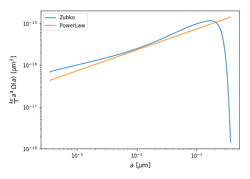
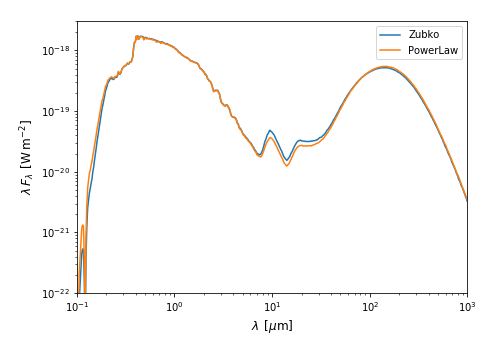
The figure on the left below shows the two grain size distributions (in volume units) plotted from the files produced by the probes "3". These probes register the bare size distributions without the front factor, so we added this factor in the plotting routine. The figure on the right shows the corresponding observed spectra.

Grain size distribution in volume units	Corresponding observed spectrum

While experimenting with the form and range of a size distribution, it is often desirable to keep the dust mass per hydrogen atom of the population constant so that the relative contribution of the population in the complete dust mix remains fixed. To achieve this, the proportionality factor must be recalculated after each change to the size distribution. To avoid this annoyance, SKIRT offers an alternative "normalization" mechanism that allows directly specifying the dust mass per hydrogen atom or per hydrogen mass of a population. Thus, for our silicate model, the following three lines in the ski file result in exactly the same grain population:

<GrainPopulation numSizes="15" normalizationType="FactorOnSizeDistribution" factorOnSizeDistribution="5.4765902385e-31">
    ... or ...
<GrainPopulation numSizes="15" normalizationType="DustMassPerHydrogenAtom" dustMassPerHydrogenAtom="8.115005680e-30 kg">
    ... or ...
<GrainPopulation numSizes="15" normalizationType="DustMassPerHydrogenMass" dustMassPerHydrogenMass="4.851668068e-03">

These alternatives are especially handy when the characteristics for a grain population are specified in these terms in the literature.

Working with grain compositions

SKIRT offers various built-in grain compositions (i.e. grain material types), including:

• the classic Draine et al. (amorphous) silicates, graphites and PAHs we have been using so far in this tutorial,
• crystalline Enstatite and Forsterite silicates prepared by Michiel Min et al.,
• a suite of material types taken from the data supplied with the DustEM code (Compiègne et al.), including more recent versions of Draine et al. silicates, graphites and PAHs; carbonaceous grains defined by Jones et al.; and amorphous olivine and pyroxene silicates defined by Koehler et al.

More information can be found in the respective class descriptions.

As an example, let us consider the THEMIS dust model. This model is already available as a turn-key dust mix in SKIRT, however it is informative to configure it as a custom dust mix in the ski file. The following is an extract from the input file specifying this dust model for the DustEM code:

# grain type, nsize, type keywords, Mdust/MH, rho, amin, amax, alpha/a0 [, at, ac, gamma (ED)] [, au, zeta, eta (CV)]
# cgs units
aOLM5  100 logn      0.255E-02  2.190E+00  1.00E-07   4900.0E-07     8.00E-07    1.00E+00
aPyM5  100 logn      0.255E-02  2.190E+00  1.00E-07   4900.0E-07     8.00E-07    1.00E+00
CM20   100 logn      0.600E-03  1.510E+00  0.50E-07   4900.0E-07     7.00E-07    1.00E+00
CM20   100 plaw-ed   0.170E-02  1.600E+00  0.40E-07   4900.0E-07    -5.00E-00   10.00E-07   50.0E-07  1.000E+00

The four grain populations use olivine, pyroxene, and carbonaceous grains (twice) with log-normal or modified power-law size distributions. These size distributions are "normalized" by specifying the dust mass per hydrogen mass (Mdust/MH). The bulk mass density is explicitly given for each material type (rho). The remaining columns provide parameters for the range and form of the size distributions.

Here is the corresponding dust mix configuration in SKIRT. The concepts and values translate quite easily, although, admittedly, the ski file version is a lot more verbose:

<ConfigurableDustMix scatteringType="HenyeyGreenstein">
    <populations type="GrainPopulation">
        <GrainPopulation numSizes="15" normalizationType="DustMassPerHydrogenMass"
                         dustMassPerHydrogenMass="0.255E-02">
            <composition type="GrainComposition">
                <DustEmGrainComposition grainType="aOlM5" bulkMassDensity="2.190E+00 g/cm3"/>
            </composition>
            <sizeDistribution type="GrainSizeDistribution">
                <LogNormalGrainSizeDistribution minSize="1.00E-07 cm" maxSize="4900.0E-07 cm"
                                                centroid="8.00E-07 cm" width="1.00E+00"/>
            </sizeDistribution>
        </GrainPopulation>
        <GrainPopulation numSizes="15" normalizationType="DustMassPerHydrogenMass"
                         dustMassPerHydrogenMass="0.255E-02">
            <composition type="GrainComposition">
                <DustEmGrainComposition grainType="aPyM5" bulkMassDensity="2.190E+00 g/cm3"/>
            </composition>
            <sizeDistribution type="GrainSizeDistribution">
                <LogNormalGrainSizeDistribution minSize="1.00E-07 cm" maxSize="4900.0E-07 cm"
                                                centroid="8.00E-07 cm" width="1.00E+00"/>
            </sizeDistribution>
        </GrainPopulation>
        <GrainPopulation numSizes="15" normalizationType="DustMassPerHydrogenMass"
                         dustMassPerHydrogenMass="0.600E-03">
            <composition type="GrainComposition">
                <DustEmGrainComposition grainType="CM20" bulkMassDensity="1.510E+00 g/cm3"/>
            </composition>
            <sizeDistribution type="GrainSizeDistribution">
                <LogNormalGrainSizeDistribution minSize="0.50E-07 cm" maxSize="4900.0E-07 cm"
                                                centroid="7.00E-07 cm" width="1.00E+00"/>
            </sizeDistribution>
        </GrainPopulation>
        <GrainPopulation numSizes="15" normalizationType="DustMassPerHydrogenMass"
                         dustMassPerHydrogenMass="0.170E-02">
            <composition type="GrainComposition">
                <DustEmGrainComposition grainType="CM20" bulkMassDensity="1.600E+00 g/cm3"/>
            </composition>
            <sizeDistribution type="GrainSizeDistribution">
                <ModifiedPowerLawGrainSizeDistribution minSize="0.40E-07 cm" maxSize="4900.0E-07 cm"
                            powerLawIndex="-5.00E-00" turnOffPoint="10.00E-07 cm"
                            scaleExponentialDecay="50.0E-07 cm" exponentExponentialDecay="1.000E+00"
                            strengthCurvature="0"/>
            </sizeDistribution>
        </GrainPopulation>
    </populations>
</ConfigurableDustMix>

Using polarization and material phase functions

Depending on the data supplied with the included dust grain compositions, a ConfigurableDustMix may support one or more of the following spherical-grain scattering mechanisms (specified with the scatteringType attribute):

• HenyeyGreenstein: the Henyey-Greenstein scattering phase function is widely used for dust scattering in an astrophysical context because it requires only a single (wavelength-dependent) parameter, namely $g=⟨\cos \theta ⟩$, the average cosine of the scattering angle $\theta$. The resulting analytical phase function form is, however, not always an excellent approximation of the actual phase function.
• SphericalPolarization: with scattering for polarized radiation, the phase function depends on the polarization state of the incoming radiation, and the polarization state of the outgoing radiation is updated appropriately. The phase function is computed from the (wavelength and grain size-dependent) coefficients of the Mueller matrix supplied for the grain composition.
• MaterialPhaseFunction: this mode calculates the actual material phase function from (part of) the Mueller matrix components supplied for the grain composition, without handling polarized radiation.

All grain compositions mentioned so far in this tutorial work with the Henyey-Greenstein scattering mode and don't support the other modes. Apart from some special-purpose dust mixes intended for use with benchmarks, only the PolarizedSilicateGrainComposition and PolarizedGraphiteGrainComposition provide the Mueller matrix data necessary to support the SphericalPolarization or MaterialPhaseFunction modes.

Configuring multiple medium components

In the configurations studied above, all grain populations under consideration are included in a single dust mix, which in turn is attached to a geometry that defines the spatial dust density distribution. This implies that the dust properties are the same everywhere in the model. We can overcome this limitation by configuring multiple media components, each with their own geometry and dust mix. For example, assume that the original dust mix has a silicate and a graphite grain population. We can then include the silicate population in the dust mix of the first medium component and the graphite population in the dust mix of the second medium component. Remember that we also need to adjust the normalization of the dust mass for each medium component to reflect the relative contribution of silicates and graphites. We can then control the spatial distribution for silicates and graphites separately by configuring different geometries for each medium component.

While this approach works perfectly for simple geometric or even imported models, it becomes unwieldy when the density distributions for a nontrivial number of separate grain populations are being imported from hydrodynamical snapshot data. This use case is discussed in the second part of this tutorial.

Spatially varying the dust mix in imported models

Reference model

In the second part of the tutorial we use SKIRT models that read both the source and medium setup from smoothed particle data provided as column text files. Rather than supplying data derived from an actual hydrodynamical simulation snapshot, we manually construct simple input data files that illustrate the concepts under study.

We first construct a reference model that we can use as the basis for further exploration. The model includes three identical sources lined up on the x-axis. Each source is embedded in a blob of dust that may have different properties. In the reference model we use a single dust mix; the only difference between the blobs is their mass. By smartly positioning a frame instrument so that each pixel covers a single source/blob combination, we can we evaluate the extinction characteristics for each dust blob separately.

The following column text data file defines the three sources for our model; this file will remain unchanged for all models considered in this tutorial:

# sources.txt
# Column 1: position x (pc)
# Column 2: position y (pc)
# Column 3: position z (pc)
# Column 4: smoothing length (pc)
# Column 5: blackbody radius (km)
# Column 6: blackbody temperature (K)
-0.66666 0  0  0.001  1e3   12000
 0       0  0  0.001  1e3   12000
 0.66666 0  0  0.001  1e3   12000

The column information in the header is optional but highly recommended. Apart from explicitly declaring the units for the tabulated quantities, the column names are reproduced in the SKIRT log file, providing an additional sanity check on the imported data. The luminosity and spectrum of the sources are specified through the radius and temperature of a blackbody emitter.

The following column text data file defines the three dust blobs enveloping the sources in our model; the contents of this file will vary along with the ski file during our further exploration:

# dust1.txt
# Column 1: position x (pc)
# Column 2: position y (pc)
# Column 3: position z (pc)
# Column 4: smoothing length (pc)
# Column 5: dust mass (Msun)
-0.66666 0  0  0.3  0.01
 0       0  0  0.3  0.02
 0.66666 0  0  0.3  0.03

The ski file configures source and media components by importing these data files:

<?xml version="1.0" encoding="UTF-8"?>
<!-- A SKIRT parameter file © Astronomical Observatory, Ghent University -->
<skirt-simulation-hierarchy type="MonteCarloSimulation" format="9">
    <MonteCarloSimulation userLevel="Regular" simulationMode="ExtinctionOnly" numPackets="5e6">
        <units type="Units">
            <ExtragalacticUnits fluxOutputStyle="Frequency"/>
        </units>
        <sourceSystem type="SourceSystem">
            <SourceSystem minWavelength="0.09 micron" maxWavelength="1.2 micron">
                <sources type="Source">
                    <ParticleSource filename="sources.txt">
                        <smoothingKernel type="SmoothingKernel">
                            <CubicSplineSmoothingKernel/>
                        </smoothingKernel>
                        <sedFamily type="SEDFamily">
                            <BlackBodySEDFamily/>
                        </sedFamily>
                    </ParticleSource>
                </sources>
            </SourceSystem>
        </sourceSystem>
        <mediumSystem type="MediumSystem">
            <MediumSystem>
                <media type="Medium">
                    <ParticleMedium filename="dust1.txt" massFraction="1">
                        <smoothingKernel type="SmoothingKernel">
                            <CubicSplineSmoothingKernel/>
                        </smoothingKernel>
                        <materialMix type="MaterialMix">
                            <ZubkoDustMix numSilicateSizes="15" numGraphiteSizes="15" numPAHSizes="10"/>
                        </materialMix>
                    </ParticleMedium>
                </media>
                <grid type="SpatialGrid">
                    <CartesianSpatialGrid minX="-1 pc" maxX="1 pc" minY="-1 pc" maxY="1 pc" minZ="-1 pc" maxZ="1 pc">
                        <meshX type="MoveableMesh">
                            <LinMesh numBins="60"/>
                        </meshX>
                        <meshY type="MoveableMesh">
                            <LinMesh numBins="60"/>
                        </meshY>
                        <meshZ type="MoveableMesh">
                            <LinMesh numBins="60"/>
                        </meshZ>
                    </CartesianSpatialGrid>
                </grid>
            </MediumSystem>
        </mediumSystem>
        <instrumentSystem type="InstrumentSystem">
            <InstrumentSystem>
                <defaultWavelengthGrid type="WavelengthGrid">
                    <LogWavelengthGrid minWavelength="0.09 micron" maxWavelength="1.2 micron" numWavelengths="100"/>
                </defaultWavelengthGrid>
                <instruments type="Instrument">
                    <FrameInstrument instrumentName="xy" distance="1 kpc"
                                     inclination="0 deg" azimuth="0 deg" roll="90 deg"
                                     fieldOfViewX="2 pc" numPixelsX="3" centerX="0 pc"
                                     fieldOfViewY="0.66666 pc" numPixelsY="1" centerY="0 pc"
                                     recordComponents="true"/>
                </instruments>
            </InstrumentSystem>
        </instrumentSystem>
        <probeSystem type="ProbeSystem">
            <ProbeSystem>
                <probes type="Probe">
                    <ConvergenceInfoProbe probeName="cnv" wavelength="0.55 micron"/>
                    <ConvergenceCutsProbe probeName="dns"/>
                </probes>
            </ProbeSystem>
        </probeSystem>
    </MonteCarloSimulation>
</skirt-simulation-hierarchy>

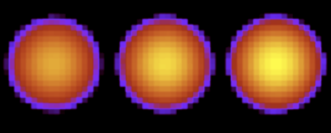
A cut through the gridded dust density along the xy plane shows the dust blobs listed in the imported file from left to right:

Cut through the density distribution of the reference model

The configured frame instrument looks down on the xy plane and has three pixels, each covering one of the source/dust combinations. The instrument records separate flux components, including the transparent flux (i.e. as if there were no dust) and the direct flux (i.e. the extincted flux ignoring scattering into the sight line). This means we can plot the effect of the dust extinction for each of the blobs separately:

Spectra for each source/dust combination in the reference model

Clearly this is a contrived setup, but it allows us to explore SKIRT's capabilities for spatially varying the dust mix in a simulation.

Multiple particle types

In the reference model, the imported particles are all of the same type and specify a single dust mass. Now consider a situation where there are multiple particle types corresponding to a different dust mix. For example, some particles represent silicate dust, and other particles represent graphite dust. Each particle still carries a single dust mass. This would lead to an import data file of the following form, with a zero-based index indicating the particle type:

# dust2.txt
# Column 1: position x (pc)
# Column 2: position y (pc)
# Column 3: position z (pc)
# Column 4: smoothing length (pc)
# Column 5: dust mass (Msun)
# Column 6: dust mix index (1)
-0.66666 0  0  0.3  0.02   1
 0       0  0  0.3  0.02   0
 0.66666 0  0  0.3  0.03   1

We address this situation in the ski file through the SelectDustMixFamily class, which uses the extra index to select one of the dust mixes listed in its dustMixes property. Other than replacing ZubkoDustMix by SelectDustMixFamily, we need to enable import of the extra column by setting the importVariableMixParams attribute of the ParticleMedium to true. Using the silicate and graphite components of the Zubko dust mix discussed in the first part of this tutorial, this leads to:

<ParticleMedium filename="dust2.txt" massFraction="1" importVariableMixParams="true">
    <smoothingKernel type="SmoothingKernel">
        <CubicSplineSmoothingKernel/>
    </smoothingKernel>
    <materialMixFamily type="MaterialMixFamily">
        <SelectDustMixFamily>
            <dustMixes type="DustMix">

                <ConfigurableDustMix scatteringType="HenyeyGreenstein">
                    <populations type="GrainPopulation">
                        <GrainPopulation numSizes="15" normalizationType="FactorOnSizeDistribution"
                                         factorOnSizeDistribution="1">
                            <composition type="GrainComposition">
                                <DraineSilicateGrainComposition/>
                            </composition>
                            <sizeDistribution type="GrainSizeDistribution">
                                <ZubkoSilicateGrainSizeDistribution/>
                            </sizeDistribution>
                        </GrainPopulation>
                    </populations>
                </ConfigurableDustMix>

                <ConfigurableDustMix scatteringType="HenyeyGreenstein">
                    <populations type="GrainPopulation">
                        <GrainPopulation numSizes="15" normalizationType="FactorOnSizeDistribution"
                                         factorOnSizeDistribution="1">
                            <composition type="GrainComposition">
                                <DraineGraphiteGrainComposition/>
                            </composition>
                            <sizeDistribution type="GrainSizeDistribution">
                                <ZubkoGraphiteGrainSizeDistribution/>
                            </sizeDistribution>
                        </GrainPopulation>
                    </populations>
                </ConfigurableDustMix>

            </dustMixes>
        </SelectDustMixFamily>
    </materialMixFamily>
</ParticleMedium>

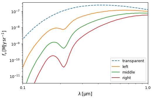
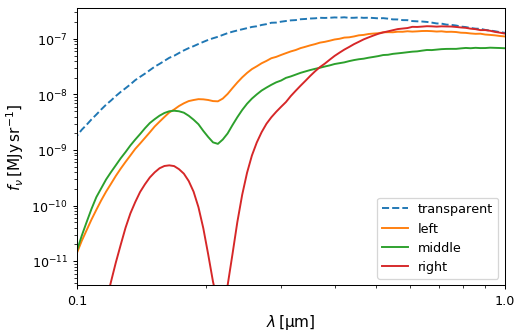
The adjusted ski file produces the following spectra. The middle dust blob contains only silicate so it does not show the graphite absorption feature. The other two blobs contain only graphite and thus they show the graphite absorption feature, at two different column densities:

Spectra for the model with multiple particle types

Masses per type of dust

A related but different situation arises when each of the imported particles carries multiple dust masses, one for each type of dust in the simulation. Consider an example with three dust types; silicates, graphite, and neutral PAHs:

# dust3.txt
# Column 1: position x (pc)
# Column 2: position y (pc)
# Column 3: position z (pc)
# Column 4: smoothing length (pc)
# Column 5: silicate mass (Msun)
# Column 6: graphite mass (Msun)
# Column 7: PAH mass (Msun)
-0.66666 0  0  0.3   0.010  0.001  0.001
 0       0  0  0.3   0.001  0.010  0.000
 0.66666 0  0  0.3   0.001  0.000  0.010

This situation can be addressed by configuring a separate medium component for each type of dust. Each medium component imports the same particles from the same file but picks the mass column that corresponds to the dust mix assigned to the component. This can be achieved through the useColumns attribute of the ParticleMedium class. The definition of the medium components now becomes:

<ParticleMedium filename="dust3.txt" massFraction="1"
                useColumns="position x,position y,position z,smoothing length,silicate mass">
    <smoothingKernel type="SmoothingKernel">
        <CubicSplineSmoothingKernel/>
    </smoothingKernel>
    <materialMix type="MaterialMix">
        <ConfigurableDustMix scatteringType="HenyeyGreenstein">
            <populations type="GrainPopulation">
                <GrainPopulation numSizes="15" normalizationType="FactorOnSizeDistribution"
                                 factorOnSizeDistribution="1">
                    <composition type="GrainComposition">
                        <DraineSilicateGrainComposition/>
                    </composition>
                    <sizeDistribution type="GrainSizeDistribution">
                        <ZubkoSilicateGrainSizeDistribution/>
                    </sizeDistribution>
                </GrainPopulation>
            </populations>
        </ConfigurableDustMix>
    </materialMix>
</ParticleMedium>

<ParticleMedium filename="dust3.txt" massFraction="1"
                useColumns="position x,position y,position z,smoothing length,graphite mass">
    <smoothingKernel type="SmoothingKernel">
        <CubicSplineSmoothingKernel/>
    </smoothingKernel>
    <materialMix type="MaterialMix">
        <ConfigurableDustMix scatteringType="HenyeyGreenstein">
            <populations type="GrainPopulation">
                <GrainPopulation numSizes="15" normalizationType="FactorOnSizeDistribution"
                                 factorOnSizeDistribution="1">
                    <composition type="GrainComposition">
                        <DraineGraphiteGrainComposition/>
                    </composition>
                    <sizeDistribution type="GrainSizeDistribution">
                        <ZubkoGraphiteGrainSizeDistribution/>
                    </sizeDistribution>
                </GrainPopulation>
            </populations>
        </ConfigurableDustMix>
    </materialMix>
</ParticleMedium>

<ParticleMedium filename="dust3.txt" massFraction="1"
                useColumns="position x,position y,position z,smoothing length,PAH mass">
   <smoothingKernel type="SmoothingKernel">
        <CubicSplineSmoothingKernel/>
    </smoothingKernel>
    <materialMix type="MaterialMix">
        <ConfigurableDustMix scatteringType="HenyeyGreenstein">
            <populations type="GrainPopulation">
                <GrainPopulation numSizes="10" normalizationType="FactorOnSizeDistribution"
                                 factorOnSizeDistribution="1">
                    <composition type="GrainComposition">
                        <DraineNeutralPAHGrainComposition/>
                    </composition>
                    <sizeDistribution type="GrainSizeDistribution">
                        <ZubkoPAHGrainSizeDistribution/>
                    </sizeDistribution>
                </GrainPopulation>
            </populations>
        </ConfigurableDustMix>
    </materialMix>
</ParticleMedium>

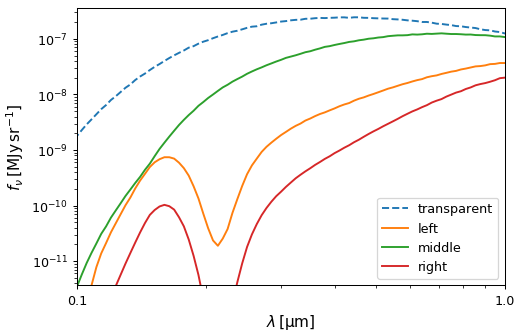
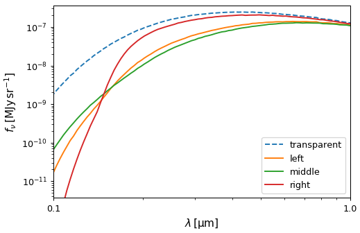
The ski file now produces the following spectra. The extinction curves have a distinct shape (other than just a scaling), indicating that the three blobs contain a different mixture of grain types.

Spectra for the model with masses per type of dust

Weights per type of dust

An alternative method achieving a similar goal is offered by the FragmentDustMixDecorator, which splits a given dust mix into its constituent fragments. The configuration now contains a single medium component with a single underlying dust mix, which is "fragmented" into its individual dust grain populations:

<ParticleMedium filename="dust4.txt" massFraction="1">
    <smoothingKernel type="SmoothingKernel">
        <CubicSplineSmoothingKernel/>
    </smoothingKernel>
    <materialMix type="MaterialMix">
        <FragmentDustMixDecorator fragmentSizeBins="false">
            <dustMix type="MultiGrainDustMix">
                <ConfigurableDustMix scatteringType="HenyeyGreenstein">
                    <populations type="GrainPopulation">
                        <GrainPopulation numSizes="15" normalizationType="FactorOnSizeDistribution"
                                         factorOnSizeDistribution="1">
                            <composition type="GrainComposition">
                                <DraineSilicateGrainComposition/>
                            </composition>
                            <sizeDistribution type="GrainSizeDistribution">
                                <ZubkoSilicateGrainSizeDistribution/>
                            </sizeDistribution>
                        </GrainPopulation>
                        <GrainPopulation numSizes="15" normalizationType="FactorOnSizeDistribution"
                                         factorOnSizeDistribution="1">
                            <composition type="GrainComposition">
                                <DraineGraphiteGrainComposition/>
                            </composition>
                            <sizeDistribution type="GrainSizeDistribution">
                                <ZubkoGraphiteGrainSizeDistribution/>
                            </sizeDistribution>
                        </GrainPopulation>
                        <GrainPopulation numSizes="10" normalizationType="FactorOnSizeDistribution"
                                         factorOnSizeDistribution="1">
                            <composition type="GrainComposition">
                                <DraineNeutralPAHGrainComposition/>
                            </composition>
                            <sizeDistribution type="GrainSizeDistribution">
                                <ZubkoPAHGrainSizeDistribution/>
                            </sizeDistribution>
                        </GrainPopulation>
                    </populations>
                </ConfigurableDustMix>
            </dustMix>
        </FragmentDustMixDecorator>
    </materialMix>
</ParticleMedium>

The import file now contains a column specifying the total mass for each particle in addition to columns specifying a weight for each of the grain populations or "fragments" in the fragmented dust mix. The order of the weights in the import file matches the order of the grain populations in the ski file. A weight of 1 indicates that the fragment will be present with its contribution to the dust mix as configured in the ski file. For example, to reproduce the result of the reference configuration (first section of this second part in the tutorial with import file "dust1.txt"), we would provide the following import file:

# dust4.txt
# Column 1: position x (pc)
# Column 2: position y (pc)
# Column 3: position z (pc)
# Column 4: smoothing length (pc)
# Column 5: total mass (Msun)
# Column 6: silicate weight (1)
# Column 7: graphite weight (1)
# Column 8: PAH weight (1)
-0.66666 0  0  0.3   0.01  1  1  1
 0       0  0  0.3   0.02  1  1  1
 0.66666 0  0  0.3   0.03  1  1  1

More generally, the contribution of a fragment is multiplied by its corresponding weight factor, allowing to spatially vary the dust mix. Assuming a configured dust mix including fragments $c$ with cross sections per hydrogen atom ${\varsigma }_c$, and given the imported weights $w_c$, the opacity $k$ of the dust in the corresponding particle is calculated as:

$$k\propto \sum _c{w}_c{\varsigma }_c,$$

where the proportionality factor is determined by the total mass and volume of the imported particle. Consequently, adjusting one or more weights affects the opacity of the dust in the corresponding particle. Also, because the wavelength-dependence of the cross section differs between the various fragments, the effect on opacity is wavelength-dependent.

If we want to control the precise fraction of the dust mass allocated to each fragment, things get a bit more involved. Because the weights specified in the import file are multiplication factors "on top of" the grain populations configured in the ski file, we need to compensate for the original mass fraction of each population in the complete dust mix. Assuming a configured dust mix including fragments $c$ with dust masses per hydrogen atom ${\mu }_c$, and given the required dust mass fractions $f_c$, the weights $w_c$ to be specified in the import file can be calcuted as:

$$w_c=f_c\frac{\sum _c{\mu }_c}{{\mu }_c}.$$

The relative mass contribution ${\mu }_c/\sum _c{\mu }_c$ for each fragment in the configured dust mix can be obtained by inserting the DustGrainPopulationsProbe in the ski file. The third column of the output of this probe lists the percentage of the total dust mass contained in each grain population:

# Medium component 0 -- dust mass per hydrogen atom: 1.305623577e-29 kg
# column 1: grain population index (1)
# column 2: grain material type (-)
# column 3: dust mass as a percentage of total (%)
...
0 Draine_Silicate     62.1543 ...
1 Draine_Graphite     32.8185 ...
2 Draine_Neutral_PAH   5.0273 ...

For example, the following import file reproduces the masses and spectra of the setup in the previous section ("masses per type of dust" with import file "dust3.txt"):

# dust5.txt
# Column 1: position x (pc)
# Column 2: position y (pc)
# Column 3: position z (pc)
# Column 4: smoothing length (pc)
# Column 5: total mass (Msun)
# Column 6: silicate weight (1)
# Column 7: graphite weight (1)
# Column 8: PAH weight (1)
-0.66666 0  0  0.3   0.012   1.34075  0.25392  1.65762
 0       0  0  0.3   0.011   0.14626  2.77006  0.00000
 0.66666 0  0  0.3   0.011   0.14626  0.00000 18.08308

The mass allocated to each fragment is determined by the product of the total mass (column 5) and the corresponding weight (columns 6-8). For the radiative transfer process itself, this product is the only relevant number. However, it is strongly recommended to have the mass column specify the total mass and the weights specify the requested deviation from that mass for each grain population, as we have done in this example. This is because part of the output produced by certain probes uses just the information in the mass column, ignoring the weights. For example, the "Input" optical depth value in the output from the SpatialGridConvergenceProbe ignores the weights, while the corresponding "Gridded" values do take the weights into account.

The FragmentDustMixDecorator can also split any of the built-in turn-key dust mixes that inherit from MultiGrainDustMix. In that case, we need to know the list of grain populations defined by that dust mix, including the order of that list. This information can be obtained by looking at the source code or by investigating the output of the DustGrainPopulationsProbe. For example, the ZubkoDustMix includes four grain populations: silicates, graphites, neutral PAHs, and ionized PAHs. The latter two specify a factor of 0.5 on the same grain size distribution, so they each count for 50% of the PAHs. The import file would thus need to be equipped with an extra column.

While using a turn-key dust mix shortens the configuration file, it is slightly less "portable" because it relies on the ordering of the grain populations in the builtin dust mix. This ordering is not firmly "guaranteed" by the implementation, although it is not likely to change anytime soon for a well-established dust mix.

Weights per grain size bin

The FragmentDustMixDecorator can also split each of the grain populations in a dust mix into their grain size bins. The size bins are always spaced logarithmically and range from the smallest to the largest grain size in the size distribution configured for the grain population.

We consider a simple example with a single silicate grain population that has just three grain size bins. In the ski file, the fragmentSizeBins attribute of the fragment decorator is set to true, and the number of size bins of the silicate population is set to 3:

<ParticleMedium filename="dust6.txt" massFraction="1">
    <smoothingKernel type="SmoothingKernel">
        <CubicSplineSmoothingKernel/>
    </smoothingKernel>
    <materialMix type="MaterialMix">
        <FragmentDustMixDecorator fragmentSizeBins="true">
            <dustMix type="MultiGrainDustMix">
                <ConfigurableDustMix scatteringType="HenyeyGreenstein">
                    <populations type="GrainPopulation">
                        <GrainPopulation numSizes="3" normalizationType="FactorOnSizeDistribution"
                                         factorOnSizeDistribution="1">
                            <composition type="GrainComposition">
                                <DraineSilicateGrainComposition/>
                            </composition>
                            <sizeDistribution type="GrainSizeDistribution">
                                <ZubkoSilicateGrainSizeDistribution/>
                            </sizeDistribution>
                        </GrainPopulation>
                    </populations>
                </ConfigurableDustMix>
            </dustMix>
        </FragmentDustMixDecorator>
    </materialMix>
</ParticleMedium>

Similarly to the previous section, the import file now has a column for the total mass in addition to weight factors for each of the size bins:

# dust6.txt
# Column 1: position x (pc)
# Column 2: position y (pc)
# Column 3: position z (pc)
# Column 4: smoothing length (pc)
# Column 5: total mass (Msun)
# Column 6: bin 1 weight (1)
# Column 7: bin 2 weight (1)
# Column 8: bin 3 weight (1)
-0.66666 0  0  0.3   0.015   1     1     1
 0       0  0  0.3   0.015   0.11  0.61  1.27
 0.66666 0  0  0.3   0.015   8.22  0.61  0.15

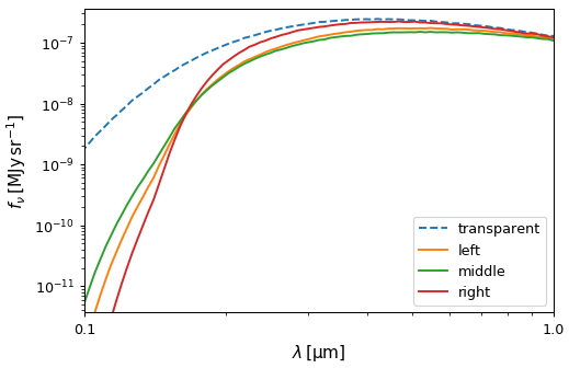
This setup produces the following spectra:

Spectra for the model with weights per grain size bin

The orange curve for the first particle matches the regular extincted spectrum for a silicate population with the configured Zubko size distribution. This can be verified by removing the fragment dust mix decorator from the ski file and running it again with the same import file. In this case, the size bin weights are ignored and the three resulting spectra are identical (and match the spectrum for the first particle with the weights specified in the import file). The second particle (green curve) is overweighted in large grains, resulting in weaker extinction at shorter wavelengths. The third particle (red curve) is overweighted in small grains, resulting in stronger extinction at shorter wavelengths.

The relative mass contribution for each size bin in the configured dust mix can again be obtained by inserting the DustGrainPopulationsProbe in the ski file (with fragment decorator):

# Medium component 0 -- dust mass per hydrogen atom: 8.115005680e-30 kg
# column 1: grain population index (1)
# column 2: grain material type (-)
# column 3: dust mass as a percentage of total (%)
...
0 Draine_Silicate   9.1213 ...
1 Draine_Silicate  24.5902 ...
2 Draine_Silicate  66.2885 ...

Using these values we can easily verify that the weights in the import file "dust6.txt" correspond to mass fractions that add up to one, i.e.

$$\sum _c{f}_c=\sum _c{w}_c{\mu }_c/\sum _c{\mu }_c\approx 1.$$

Weights per grain size bin – many bins

A hydrodynamical simulation that follows dust evolution may employ a number of grain size bins that is much larger than three. When post-processing such a simulation with SKIRT using the fragment decorator, the dust grain size distribution for each imported particle (or cell) is determined by the weights imported for each of the fairly small size bins, and the configured grain size distribution no longer really matters. However, the configured size distribution still determines the relative dust mass contributions in each of the size bins, thereby influencing the weights to be specified in the import file. We can use this fact to select a size distribution that facilitates calculating the weights.

As an example, consider a hydrodynamical simulation that uses 32 grain size bins for a single dust species, which we assume to be silicates. We expect (hope) these size bins to be spaced logarithmically, matching the spacing implemented by the fragment decorator. We set the number of size bins in the ski file to 32, and the minimum and maximum grain sizes to match the outer borders of the corresponding bins in the hydrodynamical simulation. We configure a plain power law size distribution with an exponent of 4. This ensures an identical dust mass contribution in all bins because the power law compensates for the size-dependent volume of the grains. We "normalize" the size distribution (see the first part of this tutorial) to a dust mass per hydrogen atom value that equals the value for the complete Zubko dust mix (this value can be found in the output of the DustGrainPopulationsProbe for a ski file that includes the Zubko dust mix). This results in the following ski file configuration:

<ParticleMedium filename="dust7.txt" massFraction="1">
    <smoothingKernel type="SmoothingKernel">
        <CubicSplineSmoothingKernel/>
    </smoothingKernel>
    <materialMix type="MaterialMix">
        <FragmentDustMixDecorator fragmentSizeBins="true">
            <dustMix type="MultiGrainDustMix">
                <ConfigurableDustMix scatteringType="HenyeyGreenstein">
                    <populations type="GrainPopulation">
                        <GrainPopulation numSizes="32" normalizationType="DustMassPerHydrogenAtom"
                                         dustMassPerHydrogenAtom="1.305623577e-29 kg">
                            <composition type="GrainComposition">
                                <DraineSilicateGrainComposition/>
                            </composition>
                            <sizeDistribution type="GrainSizeDistribution">
                                <PowerLawGrainSizeDistribution minSize="3.5 Angstrom" maxSize="0.35 micron"
                                                               exponent="4"/>
                            </sizeDistribution>
                        </GrainPopulation>
                    </populations>
                </ConfigurableDustMix>
            </dustMix>
        </FragmentDustMixDecorator>
    </materialMix>
</ParticleMedium>

An import file for this configuration may be:

# dust7.txt
# Column 1: position x (pc)
# Column 2: position y (pc)
# Column 3: position z (pc)
# Column 4: smoothing length (pc)
# Column 5: total mass (Msun)
# Column 6: bin 1 weight (1)
# Column 7: bin 2 weight (1)
...
# Column 37: bin 32 weight (1)
-0.66666 0  0  0.3   0.015   1 1 1 1 1 1 1 1 1 1 1 1 1 1 1 1 1 1 1 1 1 1 1 1 1 1 1 1 1 1 1 1
 0       0  0  0.3   0.015   0 0 0 0 1 1 1 1 1 1 1 1 1 1 1 1 1 1 1 1 1 1 1 1 1 1 1 1 2 2 2 2
 0.66666 0  0  0.3   0.015   3 3 3 3 1 1 1 1 1 1 1 1 1 1 1 1 1 1 1 1 1 1 1 1 0 0 0 0 0 0 0 0

From the output of the DustGrainPopulationsProbe for this setup, it can easily be verified that all fragments (or size bins) carry the same dust mass contribution. Denoting the number of size bins as $C$ (i.e. $C=32$ in our example), the formula for calculating the weigths from a given required mass fraction therefore simplifies to

$$w_c=f_{c}C.$$

This setup produces the following spectra, with similar effects as those in the previous section. The second particle (green curve) is overweighted in large grains, resulting in weaker extinction at shorter wavelengths. The third particle (red curve) is overweighted in small grains, resulting in stronger extinction at shorter wavelengths.

Spectra for the model with weights per grain size bin – many bins

It is also possible that the hydrodynamical simulation tracks the number of dust grains in each size bin (as opposed to the dust mass or mass fraction per bin). We can then set the power-law exponent of the configured dust distribution to 1, which causes the relative mass contribution of each bin to be proportional to the mass of a single grain in that bin. The weights in the import file can then be calculated directly from the number fractions (as opposed to the mass fractions) for each bin.