 |
The SKIRT project
advanced radiative transfer for astrophysics
|
|
The SKIRT project
advanced radiative transfer for astrophysics
|
SKIRT employs a spatial grid to discretize the transfer medium of the model. Properties such as the material density and the calculated radiation field are considered to be uniform within each cell of the dust grid. In this tutorial you will experiment with adaptive grids for a spiral galaxy model in SKIRT, and learn how to balance several conflicting requirements to obtain an 'optimal' grid for your purposes.
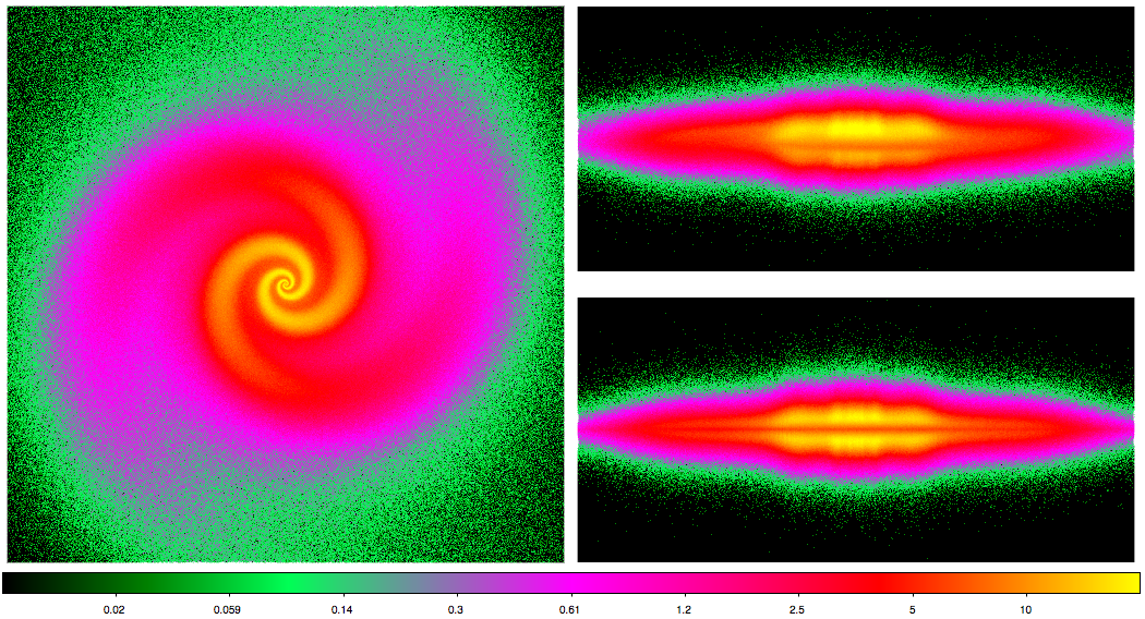
Illustration above: surface brightness of the spiral galaxy modeled in this tutorial for inclinations of 0 degrees (face-on), 86 degrees, and 90 degrees (edge-on).
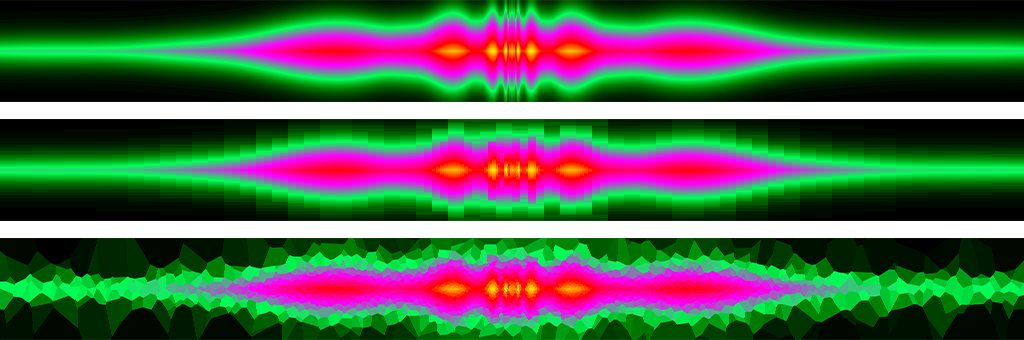
Illustration above: cut along the \(xz\)-plane through the theoretical dust density (top), the dust density gridded by an octree with 900,000 cells (middle), and the dust density gridded by a Voronoi tessellation with 200,000 cells.
This tutorial assumes that you have completed the introductory SKIRT tutorials Monochromatic simulation of a dusty disk galaxy and Stochastic heating in an SPH-simulated galaxy, or that you have otherwise acquired the working knowledge introduced there. At the very least, before starting this tutorial, you should have installed the SKIRT code, and preferably also PTS and a FITS file viewer such as DS9 (see Installation Guide).
As a first step, you need to configure a spiral galaxy model that you can then use to study the adaptive grids offered by SKIRT. In a terminal window, with an appropriate current directory, start SKIRT without any command line arguments. SKIRT responds with a welcome message and starts an interactive session in the terminal window, during which it will prompt you for all the information describing a particular simulation:
   Welcome to SKIRT v___
   Running on ___ for ___
   Interactively constructing a simulation...
 ? Enter the name of the ski file to be created: ArmedSpiralTree
The first question is for the filename of the ski file. For this tutorial, enter "ArmedSpiralTree".
In this and subsequent tutorials, we skip the questions for which there is only one possible answer. The answers to these questions are provided without prompting the user, and listing them here would bring no added value.
   Possible choices for the user experience level:
      1. Basic: for beginning users (hides many options)
      2. Regular: for regular users (hides esoteric options)
      3. Expert: for expert users (hides no options)
 ? Enter one of these numbers [1,3] (2): 1
As discussed in a previous tutorial (see Experience level), the Q&A session can be tailored to the experience level of the user. For this tutorial, select the Basic level.
   Possible choices for the units system:
      1. SI units
      2. Stellar units (length in AU, distance in pc)
      3. Extragalactic units (length in pc, distance in Mpc)
 ? Enter one of these numbers [1,3] (3):
   Possible choices for the output style for wavelengths:
      1. As photon wavelength: λ
      2. As photon frequency: ν
      3. As photon energy: E
 ? Enter one of these numbers [1,3] (1):
   Possible choices for the output style for flux density and surface brightness:
      1. Neutral: λ F_λ = ν F_ν
      2. Per unit of wavelength: F_λ
      3. Per unit of frequency: F_ν
      4. Counts per unit of energy: F_E
  ? Enter one of these numbers [1,4] (3):
As discussed in a previous tutorial (see Units), SKIRT offers several output unit options. For the current tutorial, you will be modelling a galaxy, so select extragalactic units with the wavelength output style for the spectral variable and the per unit of frequency style for fluxes (the default options).
   Possible choices for the overall simulation mode:
      1. No medium - oligochromatic regime (a few discrete wavelengths)
      2. Extinction only - oligochromatic regime (a few discrete wavelengths)
      ...
 ? Enter one of these numbers [1,8] (4): 2
As discussed in a previous tutorial (see Simulation mode), the answer to this question determines the wavelength regime of the simulation (oligochromatic or panchromatic) and sets the overall scheme for handling media in the simulation.
In an actual research setting you would probably run a panchromatic simulation to study the absorption, scattering and thermal emission by the dust over a range of wavelengths. For the purpose of studying the spatial grid in this tutorial, it is best to limit the simulation run-time by using an oligochromatic simulation at a single optical wavelength.
? Enter the default number of photon packets launched per simulation segment [0,1e19] (1e6):
To limit the run time for this tutorial, leave the number of photon packets at the default value of \(10^6\). This number is sufficient to produce an acceptable image for the simple galaxy model used here.
? Enter the wavelengths of photon packets launched from primary sources [1e-6 micron,1e6 micron] (0.55 micron): 0.55
For this tutorial enter a wavelength 'list' consisting of a single value at the center of the V-band, \(\lambda=0.55\,\mu\textrm{m}\).
   Possible choices for item #1 in the primary sources list:
      1. A primary point source
      2. A primary source with a built-in geometry
         ...
 ? Enter one of these numbers or zero to terminate the list [0,6] (2): 2
   Possible choices for the geometry of the spatial luminosity distribution for the source:
      1. A Plummer geometry
         ...
     19. A decorator that adds spiral structure to any axisymmetric geometry
     20. A decorator that adds clumpiness to any geometry
         ...
 ? Enter one of these numbers [1,21] (1): 19
   Possible choices for the axisymmetric geometry to be decorated with spiral structure:
      1. An exponential disk geometry
      2. A ring geometry
      3. A torus geometry
      4. A decorator that constructs a spheroidal variant of any spherical geometry
 ? Enter one of these numbers [1,4] (1): 1
 ? Enter the scale length ]0 pc,∞ pc[: 1800
 ? Enter the scale height ]0 pc,∞ pc[: 300
 ? Enter the radius of the central cavity [0 pc,∞ pc[ (0 pc):
 ? Enter the number of spiral arms [1,100] (1): 2
 ? Enter the pitch angle ]0 deg,90 deg[ (10 deg): 20
 ? Enter the radius zero-point ]0 pc,∞ pc[: 300
 ? Enter the weight of the spiral perturbation ]0,1]: 0.5
SKIRT offers a set of geometry "decorators" that can be used to modify other geometries in various ways. The list includes straightforward linear transformations such as translation, rotation and flattening; clipping by a sphere, cylinder or cuboid; and more complex modifications such as adding spiral arm structure or clumpiness. Decorators can be nested to arbitrary depths. In the Q&A session, you need to specify the outermost decorator first, followed by any nested decorators, and finally the original geometry being decorated.
For this tutorial, you will create a spiral galaxy model by applying the spiral structure decorator to a double-exponential disk geometry. Immediately after selecting a "built-in geometry" source component, choose the spiral structure decorator, and then choose the exponential disk geometry as the geometry to be decorated with spiral arms. SKIRT then requests the properties of the exponential disk geometry, followed by the properties of the decorator. This ordering is a consequence of the nesting mentioned above.
For the stellar exponential disk, specify a scale length of 1800 pc and a scale height of 300 pc, without an inner cavity. For the stellar spiral structure, specify 2 arms, a pitch angle of 20 degrees, a radius zero point of 300 pc, a phase zero-point of zero degrees, and a perturbation weight of 0.5.
   Possible choices for the spectral energy distribution for the source:
      1. A black-body spectral energy distribution
      2. The spectral energy distribution of the Sun
         ...
 ? Enter one of these numbers [1,9] (1): 1
 ? Enter the black body temperature ]0 K,∞ K[ (5000 K):
   Possible choices for the type of luminosity normalization for the source:
      1. Source normalization through the integrated luminosity for a given wavelength range
      2. Source normalization through the specific luminosity at a given wavelength
      3. Source normalization through the specific luminosity for a given wavelength band
 ? Enter one of these numbers [1,3] (1): 2
 ? Enter the wavelength at which to provide the specific luminosity [1e-6 micron,1e6 micron]: 0.55
   Possible choices for the luminosity unit style:
      1. Neutral: λ L_λ = ν L_ν
      2. Per unit of wavelength: L_λ
      3. Per unit of frequency: L_ν
      4. Counts per unit of energy: L_E
 ? Enter one of these numbers [1,4] (2): 2
 ? Enter the specific luminosity at the given wavelength ]0 Lsun/micron,∞ Lsun/micron[: 1e11
Because this tutorial simulation includes just a single wavelength, the emission spectrum of the source does not really matter; we just need to specify the luminosity at that wavelength. However, the Q&A questions handle the general case where both the emission spectrum and some normalization for the luminosity of each source must be specified.
For this tutorial, (arbitrarily) select a black-body spectrum with the default temperature. Then select normalization through the specific luminosity at a given wavelength, with a "per unit of wavelength" luminosity unit style. Finally, specify a luminosity at \(\lambda=0.55~\mu\text{m}\) (the wavelength specified previously) of \(L_\lambda = 10^11~\text{L}_\odot/\mu\text{m}\).
When asked for a second source component, enter zero to terminate the list.
   Possible choices for item #1 in the transfer media list:
      1. A transfer medium with a built-in geometry
         ...
 ? Enter one of these numbers [1,5] (1): 1
   Possible choices for the geometry of the spatial density distribution for the medium:
      1. A Plummer geometry
         ...
     19. A decorator that adds spiral structure to any axisymmetric geometry
         ...
 ? Enter one of these numbers [1,21] (1): 19
   Possible choices for the axisymmetric geometry to be decorated with spiral structure:
      1. An exponential disk geometry
      2. A ring geometry
      3. A torus geometry
      4. A decorator that constructs a spheroidal variant of any spherical geometry
 ? Enter one of these numbers [1,4] (1): 1
 ? Enter the scale length ]0 pc,∞ pc[: 2000
 ? Enter the scale height ]0 pc,∞ pc[: 150
 ? Enter the radius of the central cavity [0 pc,∞ pc[ (0 pc):
 ? Enter the number of spiral arms [1,100] (1): 2
 ? Enter the pitch angle ]0 deg,90 deg[ (10 deg): 20
 ? Enter the radius zero-point ]0 pc,∞ pc[: 300
 ? Enter the weight of the spiral perturbation ]0,1]: 0.5
The geometry of the spatial dust distribution can be configured in a very similar way. Select a "built-in geometry" medium component, choose the spiral structure decorator, and then choose the exponential disk geometry as the geometry to be decorated. For the dust exponential disk, specify a scale length of 2000 pc and a scale height of 150 pc, without a central cavity. For the dust spiral structure, specify 2 arms, a pitch angle of 20 degrees, a radius zero point of 300 pc, and a perturbation weight of 0.5. In other words, for this tutorial, the dust spiral structure is identical to the stellar spiral structure.
   Possible choices for the material type and properties throughout the medium:
      1. A typical interstellar dust mix (mean properties)
         ...
 ? Enter one of these numbers [1,10] (1):
   Possible choices for the type of normalization for the amount of material:
      1. Normalization by defining the total mass
      2. Normalization by defining the total number of entities
      3. Normalization by defining the optical depth along a coordinate axis
         ...
 ? Enter one of these numbers [1,5] (3): 3
   Possible choices for the axis along which to specify the normalization:
      1. The X axis of the model coordinate sytem
      2. The Y axis of the model coordinate sytem
      3. The Z axis of the model coordinate sytem
 ? Enter one of these numbers [1,3] (3): 3
 ? Enter the wavelength at which to specify the optical depth [1e-6 micron,1e6 micron]: 0.55
 ? Enter the optical depth along this axis at this wavelength ]0,∞[: 2
For this tutorial, the optical depth of the dust in the model is more important than the precise dust properties. Select the default mean interstellar dust properties with an optical depth normalization along the Z-axis at the wavelength of the simulation; specify \(\tau(0.55\,\mu\textrm{m})=2\).
When asked for a second medium component, enter zero to terminate the list.
   Possible choices for the spatial grid:
      1. A Cartesian spatial grid
      2. A tree-based spatial grid
 ? Enter one of these numbers [1,2] (2): 2
 ? Enter the start point of the box in the X direction ]-∞ pc,∞ pc[: -10 kpc
 ? Enter the end point of the box in the X direction ]-∞ pc,∞ pc[: 10 kpc
 ? Enter the start point of the box in the Y direction ]-∞ pc,∞ pc[: -10 kpc
 ? Enter the end point of the box in the Y direction ]-∞ pc,∞ pc[: 10 kpc
 ? Enter the start point of the box in the Z direction ]-∞ pc,∞ pc[: -1 kpc
 ? Enter the end point of the box in the Z direction ]-∞ pc,∞ pc[: 1 kpc
   Possible choices for the tree construction policy (configuration options):
      1. A tree grid construction policy using the medium density distribution
   Automatically selected the only choice: 1
 ? Enter the minimum level of grid refinement [0,99] (3): 2
 ? Enter the maximum level of grid refinement [0,99] (7): 6
 ? Enter the maximum fraction of dust contained in each cell [0,0.01] (1e-6): 1e-5
Consider the spatial discretization of a dust density distribution with a lot of three-dimensional structure and a large dynamic range. To obtain a rule of thumb for the resolution of a regular dust grid (i.e. a grid with fixed grid points in each dimension), one could posit that the projection of a grid cell on an instrument should have roughly the same size as a detector pixel. For a detector with only \(512\times 512\) pixels, this would lead to \(512^3\approx 1.3\times 10^8\) grid cells. However one can usually do a lot better than this. The goal is to minimize the total number of cells (and thus the simulation run time) while still producing the appropriate simulation results. To this end, it is generally best to place smaller cells in high-density areas (and in areas where the density changes rapidly), and larger cells in low-density areas. The adaptive grids offered by SKIRT serve this purpose. However, you still need to properly configure the heuristics used by these grids to place their cells.
For example, the octtree grid recursively subdivides the cuboidal domain into 8 cuboidal subcells until each cell satisfies certain criteria, or until a maximum level of subdivision has been reached. The grid can take into account several criteria other than the maximum level. The most basic criterion subdivides cells until the dust mass in each cell is smaller than a given fraction of the total dust mass in the grid. The other criteria look at the optical depth through the dust across each cell and at the dust density dispersion in each cell (a measure of the gradient in the dust density).
To start your study of adaptive grids in this tutorial, select a tree-based grid with a domain range of [-10 kpc, 10 kpc] in both the x and y directions, and a range of [-1 kpc, 1 kpc] in the z direction. Set the minimum and maximum level of refinement to 2 and 6, respectively, and set the maximum fraction of dust mass contained in each dust cell to the more relaxed value of \(10^{-5}\). You will study the effect of these parameter values in the second part of this tutorial.
   Possible choices for item #1 in the instruments list:
      1. A distant instrument that outputs the spatially integrated flux density as an SED
      2. A distant instrument that outputs the surface brightness in every pixel as a data cube
      3. A distant instrument that outputs both the flux density (SED) and surface brightness (data cube)
 ? Enter one of these numbers or zero to terminate the list [0,3] (1): 2
 ? Enter the name for this instrument: i00
 ? Enter the distance to the system ]0 Mpc,∞ Mpc[: 10
 ? Enter the inclination angle θ of the detector [0 deg,180 deg] (0 deg): 0
 ? Enter the azimuth angle φ of the detector [-360 deg,360 deg] (0 deg):
 ? Enter the total field of view in the horizontal direction ]0 pc,∞ pc[: 20 kpc
 ? Enter the number of pixels in the horizontal direction [1,10000] (250): 512
 ? Enter the total field of view in the vertical direction ]0 pc,∞ pc[: 20 kpc
 ? Enter the number of pixels in the vertical direction [1,10000] (250): 512
 ? Do you want to record flux components separately? [yes/no] (no): no
   Possible choices for item #2 in the instruments list:
      1. A distant instrument that outputs the spatially integrated flux density as an SED
      2. A distant instrument that outputs the surface brightness in every pixel as a data cube
      3. A distant instrument that outputs both the flux density (SED) and surface brightness (data cube)
 ? Enter one of these numbers or zero to terminate the list [0,3] (1): 2
 ? Enter the name for this instrument: i90
 ? Enter the distance to the system ]0 Mpc,∞ Mpc[: 10
 ? Enter the inclination angle θ of the detector [0 deg,180 deg] (0 deg): 90
 ? Enter the azimuth angle φ of the detector [-360 deg,360 deg] (0 deg):
 ? Enter the total field of view in the horizontal direction ]0 pc,∞ pc[: 20 kpc
 ? Enter the number of pixels in the horizontal direction [1,10000] (250): 512
 ? Enter the total field of view in the vertical direction ]0 pc,∞ pc[: 10 kpc
 ? Enter the number of pixels in the vertical direction [1,10000] (250): 256
 ? Do you want to record flux components separately? [yes/no] (no): no
Configure two instruments that output the total flux in every pixel, one at an inclination of 0 degrees (face-on) and one at an inclination of 90 degrees. The azimuth angles can remain at the default value of zero. The distance of the instrument to the model affects all fluxes with the same factor; use a value of your liking (for example 10 Mpc). For the face-on view, specify a field of view of \(20\times 20\) kpc centered on the origin, with \(512\times 512\) pixels. For the edge-on view, the vertical size and number of pixels can be reduced to, say, half of the horizontal size. For this tutorial, there is no reason to record flux components separately.
When asked for a third instrument, enter zero to terminate the list.
   Possible choices for item #1 in the probes list:
      1. Convergence: information on the spatial grid
      2. Convergence: cuts of the medium density along the coordinate planes
         ...
 ? Enter one of these numbers or zero to terminate the list [0,8] (1): 1
 ? Enter the name for this probe: cnv
   Possible choices for item #2 in the probes list:
      1. Convergence: information on the spatial grid
      2. Convergence: cuts of the medium density along the coordinate planes
         ...
 ? Enter one of these numbers or zero to terminate the list [0,8] (1): 2
 ? Enter the name for this probe: dns
   Possible choices for item #3 in the probes list:
      1. Convergence: information on the spatial grid
         ...
      7. Properties: data files for plotting the structure of the grid
         ...
 ? Enter one of these numbers or zero to terminate the list [0,8] (1): 7
 ? Enter the name for this probe: grd
Configure the following probes, in arbitrary order, and specify their names as follows.
| Probe type | Probe name |
|---|---|
| Convergence: information on the spatial grid | cnv |
| Convergence: cuts of the medium density along the coordinate planes | dns |
| Properties: data files for plotting the structure of the grid | grd |
After all questions have been answered, SKIRT writes out the resulting ski file and terminates. Start SKIRT again, this time specifying the name of the new ski file on the command line, to actually perform the simulation.
The output files for this tutorial are similar to those already described for a previous tutorial (see Output files and Output files). Because the geometry in this simulation is truly three-dimensional (i.e. it has no axial or spherical symmetries), there are now three cuts through the dust density (one along each of the coordinate planes) rather than two.
Open the file ArmedSpiralTree_cnv_convergence.dat in a text editor, and note the differences between the input and gridded values for the total dust mass and for the optical depth along each of the coordinate axes. The input values are calculated from the analytical expressions for the geometry of the configured dust medium; the actual values are determined by summing over the spatial grid cells. With the parameter settings given in the previous section, the discrepancy in the total dust mass is about 3%, but the optical depths show errors of up to 20%, which is not acceptable. These discrepancies are caused by a combination of two effects.
First, an exponential disk distribution extends to infinity in all directions, while the dust grid domain is necessarily finite. Thus, a portion of the dust distribution is cut off. To alleviate this issue, you can enlarge the dust grid, but that will adversely affect the total number of cells needed to resolve the dust distribution. Alternatively, you can apply cutoffs to the exponential dust distribution (by specifying these values in the geometry configuration using options that are hidden at the Basic user level), which will redistribute the clipped dust mass over the remaining part of the disk. Because the discrepancy for the total dust mass is limited in this case, it seems that this effect is limited, so no action is required.
The second cause underlying a convergence discrepancy is the discretization of the theoretical dust distribution by the cells in the spatial grid. Each cell has a uniform density determined by randomly sampling the density over the cell's volume. If there are too many large cells in areas with substantial density gradients, a discrepancy in the discretized densities will result. To help evaluate this issue, open the theoretical and gridded density cuts along the horizontal coordinate plane (ArmedSpiralTree_dns_dust_t_xy.fits and ArmedSpiralTree_dns_dust_g_xy.fits) and along one of the vertical planes (e.g. ArmedSpiralTree_dns_dust_t_xz.fits and ArmedSpiralTree_dns_dust_g_xz.fits) in a FITS file viewer such as DS9. Alternatively you can plot the density cuts using the following PTS command:
pts plot_convergence . --prefix=ArmedSpiralTree
It is worth noting that these cuts are always generated with a fixed pixel resolution of 1024 by 1024, regardless of the actual domain size. This why the vertical cuts look stretched out in a FITS viewer: the vertical size is 10 times smaller but is covered by the same number of pixels. In any case, it is obvious in the cuts that the current grid (with the parameters given in the previous section) insufficiently resolves the model's density distribution, especially near the center of the model.
It is a good idea to also review the surface brightness maps produced by the instruments, if only to verify that the instrument parameters were entered properly. If no FITS viewer is available, you can use the following PTS command to create grayscale images based on the surface brightness:
pts make_images . --prefix=ArmedSpiralTree
Even with this limited grid, the mock observations show the expected overall form. In view of the limited grid resolution, however, we can't trust the results, especially in the central areas of the model.
Now turn your attention to the simulation log messages (in the console or in the generated log file). During and immediately after constructing the octtree, SKIRT reports some statistics on the structure of the tree, similar to the following. The exact values will differ because the dust mass in a tree node is obtain by randomly sampling the density distribution.
   ...
   Constructing the spatial tree grid...
   Subdividing level 0: 1 nodes
   Subdividing level 1: 8 nodes
   Subdividing level 2: 64 nodes
   Subdividing level 3: 512 nodes
   Subdividing level 4: 3568 nodes
   Subdividing level 5: 19736 nodes
   Finished construction of the spatial tree grid
   Number of cells at each level in the tree hierarchy:
     Level  0:        0 (  0.0%)  |
     Level  1:        0 (  0.0%)  |
     Level  2:        0 (  0.0%)  |
     Level  3:       66 (  0.1%)  |
     Level  4:     1101 (  1.3%)  |
     Level  5:    10206 ( 11.6%)  |***
     Level  6:    76240 ( 87.0%)  |********************
     TOTAL   :    87613 (100.0%)
   ...
In this context, the term node indicates any node in the tree, including intermediate nodes that are subdivided and leaf nodes that are not subdivided any further. Once the tree has been constructed, the leaf nodes form the actual spatial cells of the grid.
The "Subdiving" messages are intended as a progress log. They list the number of nodes present in the tree as it has been constructed up to the indicated level. This can be helpful while fine-tuning tree construction parameters: if the number of nodes becomes excessively high, you may decide to abort the SKIRT process so that you can adjust the parameters and try again.
Once tree construction has finished, SKIRT logs the number of actual cells (i.e. leaf nodes) at each subdivision level, and it draws a rough histogram of the number of cells (asterisk bars on the horizontal axis) as a function of subdivision level (vertical axis). Level 0 corresponds to the complete spatial domain. For this simulation, there cannot be any cells at the most shallow subdivision levels (0 through 2) because the configuration specifies a minimum level of grid refinement of 2. The list ends at level 6 because the configuration specifies a maximum level of grid refinement of 6. It appears that most of the cells are at level 6, i.e. the deepest allowed subdivision level. This implies that the subdivision criteria (in this case the maximum mass fraction) are not satisfied for the majority of the dust cells. In other words, the octtree configuration is not well balanced for this particular model.
Before optimizing the dust grid, it is worth revisiting the convergence file ArmedSpiralTree_cnv_convergence.dat. At the end of that file, you will find optical depth statistics similar to the following (again, the exact values will differ because of the random density sampling process):
Optical depth of cell diagonal at 0.55 micron
  Largest: 2.73369
  Average: 0.0779654
  90% <  : 0.180564
These statistics will come in handy for setting the maximum optical depth criterion as described at the end of the following section.
The first step is to set appropriate minimum and maximum subdvision levels. The dust mass in a grid cell (or equivalently, its average dust density) is estimated by sampling the input dust density in a number of random locations across the cell volume. In low-density regions of a model, most often at its outskirts, it can happen that the sampling process "misses" the dust concentrated in one corner of a large grid cell and thus fails to trigger the maximum-mass-fraction criterion, leaving the overly large cell in place. To avoid this from happening, it is often wise to slightly increase the minimum subdvision level to a value of at least 4.
At the other end of the scale, one could use the rule of thumb mentioned earlier: the grid cells must be allowed to become at least as small as an instrument pixel (after parallel projection). Unfortunately, this provides only an upper limit on the cell size. The real question is whether the small-scale dust structure is sufficiently resolved in the grid to enable accurate calculation of the radiation field. For a semi-smooth analytical model such as the one studied in this tutorial, it seems reasonable to settle for an extra factor of two. With 512 pixels along the instrument field of view, this leads to a maximum subdvision level of \(\log_2(2*512)=10\).
Open the ArmedSpiralTree.ski file in a text editor and locate the specification of the spatial grid:
<grid type="SpatialGrid">
    <PolicyTreeSpatialGrid ... treeType="OctTree">
        <policy type="TreePolicy">
            <DensityTreePolicy minLevel="2" maxLevel="6" maxDustFraction="1e-5" maxDustOpticalDepth="0" .../>
        </policy>
    </PolicyTreeSpatialGrid>
</grid>
Adjust the minimum and maximum subdvision levels to minLevel="4" and maxLevel="10". Rerun the simulation and study the log file to evaluate the effect on the distribution of the dust cells over subdivision levels.
numPackets property at the start of the ski file). Alternatively, you can type <Ctrl>-C in the terminal window to abort SKIRT as soon as it starts shooting photon packets.With these settings the grid has slightly over 330,000 cells. There are no cells on levels 9 and 10, however. This implies that the maximum dust mass fraction criterion is too relaxed. Change this setting in the ski file from \(10^{-5}\) to \(10^{-6}\) and rerun the simulation. Now the grid has more than 3.2 million cells, most of which are on levels 8 and 9. This looks like a well-balanced grid, and for a more realistic model with a lot of small-scale clumpiness it might very well be an appropriate grid. For this tutorial (with simulations running on laptops) it is acceptable to relax the maximum mass fraction again to an intermediate value. In a more realistic research setting, one would compare the simulation results for various grids until convergence is reached. For this tutorial, you can simply pick the value of \(5\times10^{-6}\). This leads to a grid with about 650,000 cells, none of which are on level 10.
You can now further fine-tune this grid by also imposing a maximum optical depth criterion on each cell (measured across the cell diagonal). Open the convergence file and locate the optical depth statistics for your most recent grid (with min/max levels 4 and 10 and max mass fraction \(5\times10^{-6}\)). Most cells have an optical depth lower than 0.22, and some cells haven an optical depth of up to 0.63. It is beneficial for the grid quality to further subdivide the relatively small number of cells with the largest optical depths.
Set the maximum dust optical depth criterion in the ski file to a value of 0.3 (at a wavelength of \(0.55\,\mu\textrm{m}\)) and rerun the simulation. The grid now has about 900,000 grid cells, of which more than 100,000 are on level 10. In other words, the optical depth criterion added more than 30% extra cells to the grid, so that the cell optical depth distribution has a much smaller tail. Interestingly, looking at the statistics again, the largest optical depth is above the maximum optical depth criterion. This might indicate that some of the cells on level 10 have an optical depth above the maximum criterion, but could not be further subdivided because they are already at the deepest allowed level. However, this is not the case in this simulation, as can be easily verified by raising the maximum subdivision level. So what is going on?
In SKIRT, the cell mass calculations used for making subdivision decisions while constructing the tree are completely seperate from the calculations that set the cell mass in the final grid. Because the calculations sample the theoretical densities at a different set of randomly chosen locations, the results are never quite identical (except for uniform theoretical densities). The accuracy can be improved by increasing the number of random samples, at the cost of increased setup times, by changing the value of the numDensitySamples property of the SamplingOptions.
The third criterion, imposing a maximum dust density dispersion, is intended to force cell subdivisions along steep gradients in the dust density. It is applicable to geometries with clumps or dust walls that don't line up with the coordinate axes. It is not covered any further in this tutorial.
Assuming you configured the SpatialGridPlotProbe in the simulation, you can visualize the spatial grid structure with the following PTS command:
pts plot_grids . --prefix=ArmedSpiralTree
This command creates PDF files with cuts along the coordinate planes through a wireframe version of the grid such as the following (for the galactic plane of the tutorial simulation):
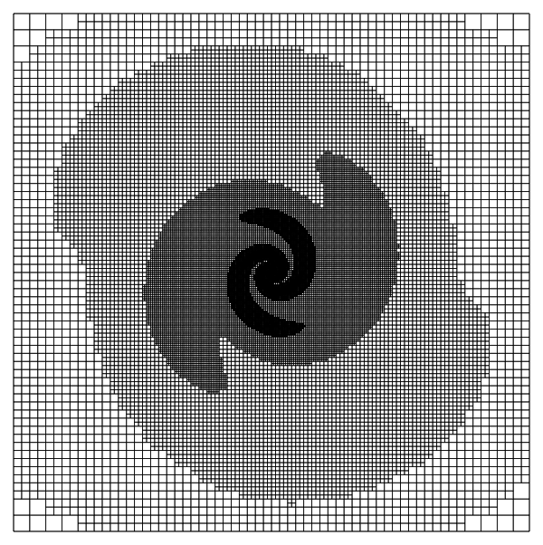
At the lower subdivision levels, the individual cells are visible. At the higher subdivision levels, the denser cells structure translates to levels of grayscale. The command also creates a three-dimensional view of the wireframe grid, which is meaningful only when the grid has very few cells (with too many cells the result is just a black blob).
As a test of your final octtree grid with 900,000 cells, you might want to run the simulation with more photon packets (e.g. \(10^7\)) and review the surface brigthness frames produced by the instruments. You could also add extra instruments at other inclinations (duplicate one of the instrument specifications in the ski file, and adjust the values for the new instrument's attributes instrumentName and inclination).
Hierarchical grids such as the octtree seem to be an obvious choice. It is fairly straightforward to construct an appropriate grid for any density field, and it is easy to calculate a straight path through the grid, since the boundaries of the cuboidal cells are lined up with the coordinate axes and each cell has a limited number of neighbors.
Hierarchical grids also have drawbacks, however. First of all, for a given density field and required resolution, an octtree grid may not be the kind of grid with the least number of cells. To illustrate this, consider a density field defined by a set of smoothed particles. An octree grid constructed such that each cell encloses at most one particle usually has over three times more cells than there are particles; i.e., two out of three cells are empty. In contrast, an unstructured grid based on a Voronoi tessellation of the spatial domain, using the given particles as generating sites, has exactly the same number of cells as there are particles. While not an issue in many situations, minimizing the number of cells is sometimes crucial. For example, consider a panchromatic radiative transfer simulation involving small dust grains in non-LTE conditions. Because each cell stores radiation field data per wavelength bin, memory requirements are substantial. Moreover, the simulation run time may very well be dominated by the calculation of the non-LTE heating and re-emission of the dust grains in each cell. In this case, both memory usage and run time scale roughly linearly with the number of cells.
Furthermore, radiative transfer simulations frequently serve to predict the observable properties of artificial systems resulting from hydrodynamical simulations. Some recent simulation codes introduce a new scheme that employs a moving mesh based on a Voronoi tessellation of the spatial domain. This new scheme is claimed to combine the best features of SPH and the traditional Eulerian approach, and it is becoming increasingly popular. While the output from a moving mesh code can be re-gridded to a hierarchical grid to perform radiative transfer, the resampling process unavoidably introduces inaccuracies and represents additional overhead. Thus it may be preferable to perform both aspects of the simulation (hydrodynamics and radiative transfer) on the same grid.
Finally, calculating a straight path through a 3D Voronoi grid is less daunting than it may seem, so that it becomes possible to perform accurate and reasonably efficient radiative transfer on unstructured Voronoi grids.
To avoid overwriting your octtree simulation results, copy the ski file ArmedSpiralTree.ski to another file called, for example, ArmedSpiralVoro.ski. Open this new file in a text editor and replace the spatial grid specification by the following:
<grid type="SpatialGrid">
    <VoronoiMeshSpatialGrid minX="-1e4 pc" maxX="1e4 pc" minY="-1e4 pc" maxY="1e4 pc" minZ="-1e3 pc" maxZ="1e3 pc"
                            policy="DustDensity" numSites="200000" relaxSites="false"/>
</grid>
Using these parameters, SKIRT will construct a Voronoi grid with 200,000 cells. The locations of the seed points or sites will be sampled from the theoretical dust density distribution. In other words, on average, the cells will be smaller in high-density regions and larger in low-density regions.
With this number of cells, the results of the SpatialGridPlotProbe are essentially meaningless (the plot becomes a black blob) and take quite some time to generate, so it is best to remove this probe from the probe list (near the end of the ski file).
After saving the above changes, run this new simulation. Shooting photons through a Voronoi grid is about three times slower than through a (highly optimized) octtree grid. The Voronoi grid may not be a big win for this monochromatic tutorial simulation, but it might still be beneficial for more complex panchromatic simulations as indicated above.
Evaluate the results of the simulation, following more or less the steps described in section Initial analysis. When comparing the simulation results between the octtree grid (with 900,000 cells) and the Voronoi grid (with 200,000 cells), take note of the following points.
The dust density discretization with the Voronoi grid is not numerically converged. The convergence metrics show optical depth discrepancies of over 10%. Probably as a result of this, the observed flux density in the central edge-on regions differs somewhat between the two simulations. However, the Voronoi grid has four times fewer cells! Given sufficient time and computing resources, you might want to increase the number of cells until the simulation results reach convergence.
All octtree cells have the same form factor as the complete domain of the grid, in this case rather flat (the height is 10 times smaller than the width), while the Voronoi cells don't have any such predisposition. This gives the octtree an advantage over the Voronoi grid in resolving the central regions of the model. More intelligent placement of the Voronoi sites might alleviate this issue. SKIRT offers schemes for placing the Voronoi sites randomly (uniform, with a steep central peak, according to dust density) or deterministically (at SPH particle locations, loaded from file) to help achieve optimal placement.
Congratulations, you made it to the end of this tutorial!