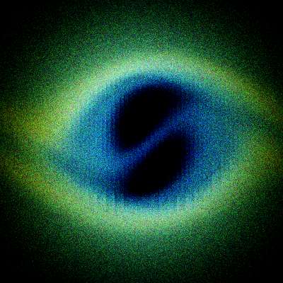
Illustration above: false-color image of the surface brightness of scattered radiation for the AMR-simulated Kelvin-Helmholtz instability used in this tutorial.

In this tutorial you will use SKIRT to study the dust in a Kelvin-Helmholtz instability as it might occur in a molecular cloud. The dust distribution has been generated by a hydrodynamical simulation on an adaptive mesh (AMR = Adaptive Mesh Refinement) with the MPI-AMRVAC code developed at the K.U.Leuven (see http://amrvac.org). The simulation includes a gas component and a dust component. The resulting spatial dust density distribution has been written to a text column file in a format appropriate for importing into SKIRT.

Getting ready

This tutorial assumes that you have completed the introductory SKIRT tutorial Monochromatic simulation of a dusty disk galaxy, or that you have otherwise acquired the working knowledge introduced there. At the very least, before starting this tutorial, you should have installed the SKIRT code, and preferably also PTS and a FITS file viewer such as DS9 (see Installation Guide).

To complete this tutorial, you need the example output file produced by the MPI-AMRVAC simulation. Download the file kh_amr.txt using the link provided in the table below and put it into your local working directory.

Dust density distribution	kh_amr.txt

Creating the ski file

Starting the SKIRT Q&A

In a terminal window, with your local working directory as the current directory, start SKIRT without any command line arguments. SKIRT responds with a welcome message and starts an interactive session in the terminal window, during which it will prompt you for all the information describing a particular simulation:

   Welcome to SKIRT v___
   Running on ___ for ___
   Interactively constructing a simulation...
 ? Enter the name of the ski file to be created: ScatAMR

The first question is for the filename of the ski file. For this tutorial, enter "ScatAMR".

In this and subsequent tutorials, we skip the questions for which there is only one possible answer. The answers to these questions are provided without prompting the user, and listing them here would bring no added value.

Experience level

   Possible choices for the user experience level:
      1. Basic: for beginning users (hides many options)
      2. Regular: for regular users (hides esoteric options)
      3. Expert: for expert users (hides no options)
 ? Enter one of these numbers [1,3] (2): 2

As discussed in a previous tutorial (see Experience level), the Q&A session can be tailored to the experience level of the user. In this tutorial, you will be using just a few features that would be hidden in the Basic level. Thus, you need to select the Regular level.

Units

   Possible choices for the units system:
      1. SI units
      2. Stellar units (length in AU, distance in pc)
      3. Extragalactic units (length in pc, distance in Mpc)
 ? Enter one of these numbers [1,3] (3): 2
   Possible choices for the output style for wavelengths:
      1. As photon wavelength: λ
      2. As photon frequency: ν
      3. As photon energy: E
 ? Enter one of these numbers [1,3] (1):
   Possible choices for the output style for flux density and surface brightness:
      1. Neutral: λ F_λ = ν F_ν
      2. Per unit of wavelength: F_λ
      3. Per unit of frequency: F_ν
      4. Counts per unit of energy: F_E
  ? Enter one of these numbers [1,4] (3):

As discussed in a previous tutorial (see Units), SKIRT offers several output unit options. For the current tutorial, you will be modelling a molecular cloud, so it is most convenient to use stellar units. You can still use any of the supported units to enter parameter values, which will be handy to avoid manual unit conversions in a few places. Thus, select stellar units with the wavelength output style for the spectral variable and per-frequency output style for fluxes, expressing integrated flux density in Jy and surface brightness in MJy/sr.

Simulation mode

   Possible choices for the overall simulation mode:
      1. No medium - oligochromatic regime (a few discrete wavelengths)
      2. Extinction only - oligochromatic regime (a few discrete wavelengths)
      ...
 ? Enter one of these numbers [1,8] (4): 2

As discussed in a previous tutorial (see Simulation mode), the answer to this question determines the wavelength regime of the simulation (oligochromatic or panchromatic) and sets the overall scheme for handling media in the simulation.

In an actual research setting you would probably run a panchromatic simulation to study the absorption, scattering and thermal emission by the dust over a range of wavelengths. In this tutorial you will simply study scattering by the dust at three specific optical wavelengths. An oligochromatic simulation is sufficient and most performance-effective for this purpose. So select the option called "Extinction only - oligochromatic regime".

Photon packets

 ? Enter the default number of photon packets launched per simulation segment [0,1e19] (1e6): 1e7

The number of photon packets must be higher than the default value to achieve an acceptable signal to noise ratio in the observed scattered radiation. To limit the run time for this tutorial, set the number of photon packets to $10^{7}$ . This number is sufficient to produce a results for this tutorial, but would likely be insufficient in an actual research setting.

Redshift

   Possible choices for the cosmology parameters:
      1. The model is at redshift zero in the Local Universe
      2. The model is at a given redshift in a flat universe
 ? Enter one of these numbers [1,2] (1):

SKIRT allows placing a simulated model at a specified nonzero redshift. For this tutorial, however, select the default option to place the model in the Local Universe.

Source system

 ? Enter the wavelengths of photon packets launched ... [1e-6 micron,1e6 micron] (0.55 micron): 0.3, 0.55, 0.8

For an oligochromatic simulation, the source system requests the list of distinct wavelengths for which to launch photon packets. For this tutorial, enter three values at the extremes and in the center of the optical wavelength range: $λ_{1, 2, 3} = 0.3, 0.55, 0.8 μ m$ . The values must be separated by commas.

   Possible choices for item #1 in the primary sources list:
      1. A primary point source
      2. A primary source with a built-in geometry
      3. A primary source imported from smoothed particle data
         ...
 ? Enter one of these numbers or zero to terminate the list [0,6] (2):
   Possible choices for the geometry of the spatial luminosity distribution for the source:
      1. A Plummer geometry
      2. A gamma geometry
         ...
 ? Enter one of these numbers [1,20] (1):
 ? Enter the scale length ]0 AU,.. AU[: 0.03e18 cm

Since the data file provided for this tutorial has no information on radiation sources, you need to configure an artificial stellar system to illuminate the dust. The suggested option is to use a Plummer profile with a scale length comparable to the size of the dust distribution (i.e. $0.03 \times 10^{18} c m$ ); this creates a nearly uniform radiation source across the configuration space.

   Possible choices for the spectral energy distribution for the source:
      1. A black-body spectral energy distribution
         ...
     12. A spectral energy distribution specified inside the configuration file
 ? Enter one of these numbers [1,12] (1): 12
 ? Enter the wavelengths at which to specify the specific luminosity [1e-6 micron,1e6 micron]: 0.2, 1
   Possible choices for the luminosity unit style:
      1. Neutral: λ L_λ = ν L_ν
      2. Per unit of wavelength: L_λ
      3. Per unit of frequency: L_ν
      4. Counts per unit of energy: L_E
 ? Enter one of these numbers [1,4] (2): 3
 ? Enter the specific luminosities at each of the given wavelengths ]0 W/Hz,∞ W/Hz[: 1, 1
   Possible choices for the type of luminosity normalization for the source:
      1. Source normalization through the integrated luminosity for a given wavelength range
      2. Source normalization through the specific luminosity at a given wavelength
      3. Source normalization through the specific luminosity for a given wavelength band
 ? Enter one of these numbers [1,3] (1): 2
 ? Enter the wavelength at which to provide the specific luminosity [1e-6 micron,1e6 micron]: 0.55
   Possible choices for the luminosity unit style:
      1. Neutral: λ L_λ = ν L_ν
      2. Per unit of wavelength: L_λ
      3. Per unit of frequency: L_ν
      4. Counts per unit of energy: L_E
 ? Enter one of these numbers [1,4] (2): 2
 ? Enter the specific luminosity at the given wavelength ]0 Lsun/micron,∞ Lsun/micron[: 1

As with any other source, you need to provide its emission spectrum and luminosity. In this tutorial, the goal is to study the effects of the wavelength-dependent dust properties, and so it is most convenient to configure the same input luminosity for each of the three wavelengths in the simulation. At the start of the configuration process you chose to output the surface brightness in "per frequency" units, so you now need to configure the input luminosities to be identical for the three wavelengths in those same "per frequency" units. This can be accomplished by configuring a custom SED, for which you can specify a tabulated functional form within the configuration file itself. You could also load a custom SED from a file, but in this case it seems overkill to create yet another input file.

Proceed as follows:

Select the "spectral energy distribution specified inside the configuration file" option.
Enter a wavelength list consisting of two wavelength points well outside of the range of the wavelengths used by this oligochromatic simulation. This will ensure that the SED is defined for all relevant wavelengths.
Select the "per frequency" style for the luminosity units.
Enter a luminosity list consisting of two identical luminosity values (for example unity). As long as both are equal, the values don't really matter because the SED will be normalized anyway (see next steps).
Select "normalization through the specific luminosity at a given wavelength".
Specify a normalization wavelength of $λ = 0.55 μ m$ .
Select the "per wavelength" style for the specific luminosity units.
Specify a the specific luminosity at that wavelength of $L_{λ} = 1 L_{⊙} / μ m$ .

There is no inconsistency in using "per frequency" style for configuring the spectrum and "per wavelength" style for the normalization. The former is to ensure a flat spectrum in the units used for output; the latter is to provide a normalization value in units that are intuitive in the context of a molecular cloud.

When asked for a second stellar component, enter zero to terminate the list.

Medium system

   Possible choices for item #1 in the transfer media list:
      1. A transfer medium with a built-in geometry
      2. A transfer medium imported from smoothed particle data
      3. A transfer medium imported from cuboidal cell data
      4. A transfer medium imported from data represented on an adaptive mesh (AMR grid)
      5. A transfer medium imported from data represented on a Voronoi mesh
 ? Enter one of these numbers [1,5] (1): 4
 ? Enter the name of the file to be imported: kh_amr.txt
 ? Enter the start point of the domain in the X direction ]-∞ AU,∞ AU[: -0.03e18 cm
 ? Enter the end point of the domain in the X direction ]-∞ AU,∞ AU[: 0.03e18 cm
 ? Enter the start point of the domain in the Y direction ]-∞ AU,∞ AU[: -0.03e18 cm
 ? Enter the end point of the domain in the Y direction ]-∞ AU,∞ AU[: 0.03e18 cm
 ? Enter the start point of the domain in the Z direction ]-∞ AU,∞ AU[: -0.03e18 cm
 ? Enter the end point of the domain in the Z direction ]-∞ AU,∞ AU[: 0.03e18 cm

For this tutorial, select a transfer medium component with a spatial distribution imported from an adaptive mesh data file, and enter the appropriate filename (kh_amr.txt). You must also provide the spatial extent of the mesh in each direction (i.e. a half-width of $0.03 \times 10^{18} c m$ centered on the origin), because this information is not included in the import data file.

   Possible choices for the type of mass quantity to be imported:
      1. Mass density
      2. Mass (volume-integrated mass density)
         ...
 ? Enter one of these numbers [1,6] (1): 1
 ? Enter the fraction of the mass to be included (or one to include all) [0,1] (1): 1e-21
 ? Do you want to import a metallicity column? [yes/no] (no):
 ? Do you want to import a temperature column? [yes/no] (no):
 ? Do you want to import parameter(s) to select a spatially varying material mix? [yes/no] (no):

Next, you need to configure the column(s) to be imported from the data file. Let us have a look at the first few lines of this file:

# Spatial dust distribution in Kelvin-Helmholtz instability extracted from MPI-AMRVAC simulation snapshot
# Converted to Adaptive Mesh import format as expected by SKIRT 9
#
# Column 1: dust mass density in units of 1e-21 g/cm3 but advertised as (g/cm3)
#
! 4 16 4
! 8 8 8
1.0227604
1.01830358

Lines starting with a hash sign (#) contain comments intended for human beings. They are generally ignored by SKIRT with the important exception that they may contain column descriptors as discussed below. Lines starting with an exclamation point describe the hierarchical structure of the AMR grid. The other lines contain information for each leaf cell; in this case, just a single column specifying the dust mass density.

The comments line starting with "Column 1" is recognized by SKIRT as a column descriptor that conveys information on the first (and only) column in the file. SKIRT recognizes and uses the units specified between parentheses. However, the values are actually given in units of $10^{- 21} g c m^{- 3}$ . The additional conversion factor of $10^{- 21}$ can be applied by specifying it as the fraction of the mass to be included. This option is actually intended to configure the fraction of metallic gas locked into dust but we can use it to implement a unit conversion factor. Alternatively, we could have adjusted the values in the input file itself.

Thus, in summary, select the "mass density" option, enter the $10^{- 21}$ factor as a mass fraction, and leave the three extra import options to their default value of "no".

   Possible choices for the material type and properties throughout the medium:
      1. A typical interstellar dust mix (mean properties)
      2. A TRUST benchmark dust mix (mean properties, optionally with polarization)
         ...
 ? Enter one of these numbers [1,19] (1):

For this tutorial, simply select the default interstellar dust mix. In an actual research setting, you would probably configure more specific dust properties.

When asked for a second medium component, enter zero to terminate the list.

Spatial grid

 ? Enter the number of random density samples for determining spatial cell mass [1,1000] (100):

This option allows configuring the number of samples taken from the spatial density distribution when determining the total dust mass in each grid cell. Leave it at the default value.

   Possible choices for the spatial grid:
      1. A Cartesian spatial grid
      2. A tree-based spatial grid
      3. A tree-based spatial grid loaded from a topology data file
      4. A spatial grid taken from an imported adaptive mesh snapshot
      5. A Voronoi tessellation-based spatial grid
 ? Enter one of these numbers [1,5] (2): 4

SKIRT discretizes the spatial domain using a grid, i.e. a collection of small cells in which properties such as dust density are considered to be uniform. You could select any of the 3D dust grids offered by SKIRT. The tree-based grid, for example, builds a grid adapted to the dust density distribution based on some given parameters. When importing a dust distribution from an adaptive mesh data file, SKIRT also offers the option to directly use the adaptive mesh defined by the data file as a spatial grid for the radiative transfer simulation. The radiative transfer grid then exactly mirrors the resolution structure of the hydrodynamical simulation, which seems a natural thing to do. On the other hand, in some cases building a new grid (perhaps with fewer cells) may prove meaningful. Indeed, the hydrodynamical simulation and the radiative transfer post-processing might have different resolution requirements. Regridding may help to place smaller cells in regions where it matters for radiaton transport, and/or to reduce the runtime of the SKIRT simulation.

For this tutorial select the option to use the imported adaptive mesh as a dust grid.

Instrument system

   Possible choices for item #1 in the instruments list:
      1. A distant instrument that outputs the spatially integrated flux density as an SED
      2. A distant instrument that outputs the surface brightness in every pixel as a data cube
      3. A distant instrument that outputs both the flux density (SED) and surface brightness (data cube)
         ...
 ? Enter one of these numbers or zero to terminate the list [0,6] (1): 2
 ? Enter the name for this instrument: xy
 ? Enter the distance to the system ]0 pc,∞ pc[: 1
 ? Enter the inclination angle θ of the detector [0 deg,180 deg] (0 deg): 0
 ? Enter the azimuth angle φ of the detector [-360 deg,360 deg] (0 deg): 0
 ? Enter the roll angle ω of the detector [-360 deg,360 deg] (0 deg): 90
 ? Enter the total field of view in the horizontal direction ]0 AU,∞ AU[: 0.06e18 cm
 ? Enter the number of pixels in the horizontal direction [1,10000] (250): 400
 ? Enter the center of the frame in the horizontal direction ]-∞ AU,∞ AU[ (0 AU):
 ? Enter the total field of view in the vertical direction ]0 AU,∞ AU[: 0.06e18 cm
 ? Enter the number of pixels in the vertical direction [1,10000] (250): 400
 ? Enter the center of the frame in the vertical direction ]-∞ AU,∞ AU[ (0 AU):
 ? Do you want to record flux components separately? [yes/no] (no): yes
 ? Enter the number of individually recorded scattering levels [0,99] (0):
 ? Do you want to record polarization (Stokes vector elements)? [yes/no] (no):
 ? Do you want to record information for calculating statistical properties? [yes/no] (no):

Since you want to study the scattered surface brightness, you need to select the surface brightness instrument and configure it to record individual contributions to the flux. Position the instrument so that it shows a projection of the $x y$ coordinate plane (angles: 0, 0, 90 degrees). This facilitates visual comparison of the recorded fluxes with the corresponding cut through the dust density produced by the corresponding probe. The distance of the instrument to the model affects all fluxes with the same factor; use a value of your liking (for example 1 pc). Setup a pixel resolution of your liking (for example $400 \times 400$ pixels) and provide a field of view that matches the size of the dust distribution to be imported. For the AMR file used in this tutorial, the size of the cubical dust distribution in each direction is $0.06 \times 10^{18}$ cm and the cube is centered on the origin.

When asked for a second instrument, enter zero to terminate the list.

Probe system

   Possible choices for item #1 in the probes list:
      1. Convergence: information on the spatial grid
      2. Convergence: cuts of the medium density along the coordinate planes
         ...
 ? Enter one of these numbers or zero to terminate the list [0,13] (1): 1
 ? Enter the name for this probe: cnv
 ? Enter the wavelength at which to determine the optical depth [1e-6 micron,1e6 micron] (0.55 micron):
   Possible choices for item #2 in the probes list:
      1. Convergence: information on the spatial grid
      2. Convergence: cuts of the medium density along the coordinate planes
         ...
 ? Enter one of these numbers or zero to terminate the list [0,13] (1): 2
 ? Enter the name for this probe: dns

Configure the following probes, in arbitrary order, and specify their names as follows.

Probe type	Probe name
Convergence: information on the spatial grid	cnv
Convergence: cuts of the medium density along the coordinate planes	dns

Finally, when asked for the subsequent probe, enter zero to terminate the list.

Performing the simulation

The simulation

After all questions have been answered, SKIRT writes out the resulting ski file and quits. Start SKIRT again, this time specifying the name of the new ski file on the command line, to actually perform the simulation. If the input data file kh_amr.txt is not in your current directory, you can specify the input directory on the SKIRT command line. For example:

skirt -i ../in ScatAMR

Output files

Most of the output files for this tutorial are similar to those already described for a previous tutorial (see Output files and Output files). This section describes the output file types that are new to this tutorial.

Because the geometry in this simulation is truly three-dimensional (i.e. it has no axial or spherical symmetries), there are now three cuts through the dust density (one along each of the coordinate planes) rather than two. Also, the instrument configured in this tutorial produces multiple files, recording various components of the observed surface brightness in separate data cubes (each including three frames, one for each wavelength):

ScatAMR_xy_total.fits contains the total surface brightness detected by the instrument; in this case, the sum of the primary direct and primary scattered components.
ScatAMR_xy_primarydirect.fits contains the surface brightness resulting from photon packets originating from the Plummer sphere that directly reach the instrument without being scattered but may be attenuated by dust absorption.
ScatAMR_xy_primaryscattered.fits contains the surface brightness resulting from photon packets originating from the Plummer sphere that were scattered by the dust at least once before reaching the instrument and may be attenuated by dust absorption.
ScatAMR_xy_transparent.fits contains the surface brightness that would be detected by the instrument if there were no medium in the system.

Dust density

As always it is a good idea to open the file ScatAMR_cnv_convergence.dat in a text editor and check the dust grid convergence metrics. For this simulation, the gridded values should be nearly identical to the input values (within numerical rounding errors) because the radiative transfer grid is identical to the grid on which the input dust density is represented.

It is also instructive to compare the theoretical and gridded dust density cuts (e.g. ScatAMR_dns_dust_t_xy.fits and PanTorus_dns_dust_g_xy.fits) in an interactive FITS viewer or by plotting them using the following PTS command:

pts plot_convergence . --prefix=ScatAMR --dex 3

Because, for this tutorial, both "input" and "gridded" values are discretized on the same spatial grid, the top and bottom rows in the figure should be identical.

Surface brightness

Open the various ScatAMR_xy_* output files in an interactive FITS file viewer.

The transparent surface brightness (ScatAMR_xy_transparent.fits) simply reflects the Plummer model used as a radiation source. It is the same for all three wavelengths, except for random noise caused by the Monte Carlo technique used in SKIRT, especially given the fairly small number of photon packets used for this simulation.

The total surface brightness (ScatAMR_xy_total.fits) shows the effects of wavelength-dependent dust extinction, but is still dominated by direct light from the Plummer source. It is more convenient to study the radiation that gets observed after having been scattered by the dust at least once, recorded by SKIRT as a separate component (ScatAMR_xy_primaryscattered.fits). The scattered surface brightness indeed shows a marked pattern that is very similar to the geometry of the dust distribution in the $x y$ plane, and that also depends on the wavelength (because the absorption and scattering cross sections of the dust vary with wavelength).

Making RGB images

Alternatively, PTS offers a command to create a regular RGB image (in PNG format) for the FITS files generated by SKIRT instruments. By default PTS uses the first FITS frame for the Blue channel, the last FITS frame for the Red channel, and some frame in the middle for the Green channel. This works well for oligochromatic simulations with 3 wavelengths such as the one in this tutorial.

To obtain an RGB image of the scattered surface brightness, enter the following command:

pts make_images . --prefix=ScatAMR --type=primaryscattered

The image file (in PNG format) is placed next to the corresponding FITS file using the same name except for the .png extension. It should look similar to the image at the start of this tutorial (see Scattering by dust in a Kelvin-Helmholtz instability), except that it will be more noisy (the image at the start of the tutorial was made with $10^{8}$ photon packets).

The colors in the image are caused by the surface brightness differences for the three wavelengths, which in turn are caused by two distinct processes:

A physical effect, because the absorption and scattering cross sections of the dust vary with wavelength.
A numerical effect, because of the random noise in the Monte Carlo technique used in SKIRT.

The latter effect is more severe for a smaller number of photon packets in the simulation.

Congratulations, you made it to the end of this tutorial!