|
The SKIRT project
advanced radiative transfer for astrophysics
|
|
The SKIRT project
advanced radiative transfer for astrophysics
|
In this tutorial, you study the polarization characteristics of the UV emission from a typical quasar using a SKIRT model that benefits from being simulated in spherical coordinates. Although you can download all ingredients to perform the simulations being discussed, the text is perhaps conceived more as a case study than as a detailed tutorial.
Along the way, you will:
This text below assumes that you have completed the introductory SKIRT tutorials Monochromatic simulation of a dusty disk galaxy and Panchromatic simulation of a dust torus, and that you have reviewed the topics on Spatial grids and meshes overview and Configuring for polarized radiation, or that you have otherwise acquired the working knowledge introduced there.
While you do not necessarily need to run any SKIRT simulations to follow along with this tutorial/case study, it certainly is instructive to review the ski files being discussed. Thus, begin by downloading the ski files using the links provided in the table below.
If you do want to perform the simulations on your system. pehaps in slightly modified form, then you should obviously have installed the SKIRT code, and preferably also PTS and a FITS file viewer such as DS9 (see Installation Guide).
| Ski file for 2D model | TutorialSpherical2D.ski |
|---|---|
| Ski file for 3D model | TutorialSpherical3Dtop.ski |
| Ski file for 3D model | TutorialSpherical3Dbot.ski |
Imagine you plan to develop a suite of SKIRT models for interpreting the (rest frame) UV polarization of so-called Blue Hot DOGs (hot dust-obscured galaxies with excess of blue emission), an intriguing subpopulation of heavily obscured quasars. You start by constructing and studying a single representative model (described here). You can subsequently vary the parameters of the model to investigate the effects of the precise geometry on the results (not described here).
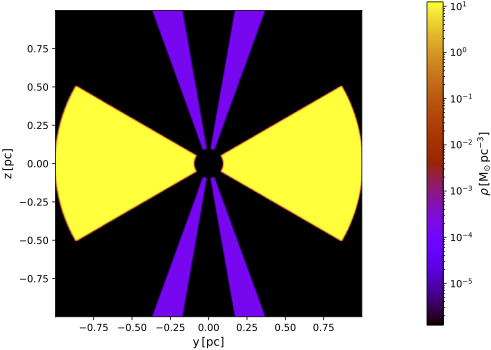
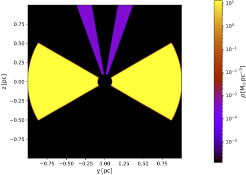
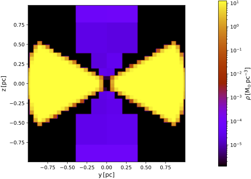
Your basic model specifies a typical configuration for an active galactic nucleus (AGN), namely a central point source surrounded by a torus and a conical shell. Since you are interested in UV polarization, the torus has a role of blocking the central source, while most of the polarization signal is produced by scattering in the cone. The illustration below shows a vertical cut through the medium density distribution. Note the large dynamic range: the cone is about 5 orders of magnitude less dense than the torus.
| Vertical cut through basic model | Vertical cut zoomed in on central portion |
|---|---|
|
|
This model is described in the TutorialSpherical2D.ski file. Open this file in a text editor and locate the various elements described below.
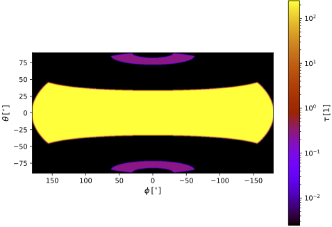
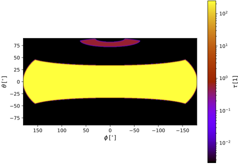
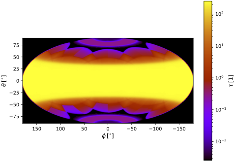
The illustration below shows an all-sky projection of the UV optical depth viewed from the model center. Note that equatorial (edge-on) sight lines show a radial optical depth of \(\tau_{0.21\mu\text{m}}>200\).
| All-sky optical depth at \(0.21~\mu\text{m}\) for basic model |
|---|
|
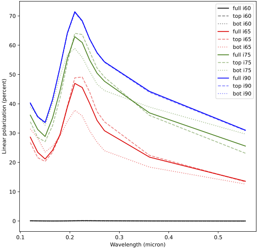
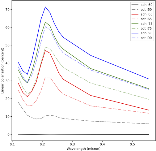
The solid lines in the plot below show the simulated linear polarization (in percent) for the four sight lines as a function of wavelength. For a definition of linear polarization, refer to Configuring for polarized radiation. Please ignore the dashed and dotted lines for now; they are discussed in the next section. The unobscured sight line (black) shows no polarization because direct emission of the unpolarized source fully dominates any scattered component. The edge-on sight line (blue) shows maximum polarization because (1) direct emission is strongly attenuated and (2) the 90 deg scattering angle from the source maximizes polarization strength.
| Polarization for models with full and half cone |
|---|
|
The observations of some of the Blue Hot DOGs under study show only a single cone. To mimick this in your SKIRT model, you employ a geometry decorator to remove the top or bottom portion of the "dual" cone. This results in two models, one with a cone pointing towards the instruments and one with a cone pointing away from the instruments. (Alternatively, you could use a single cone-configuration and add instruments at inclinations below the equatorial plane.)
The model with just the top portion of the cone is described in the TutorialSpherical3Dtop.ski file. Open this file in a text editor and review the differences with the original model as described below.
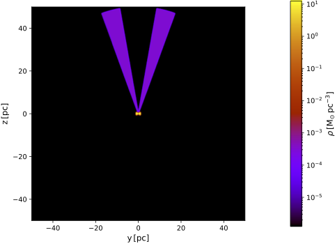
The illustrations below show the vertical cuts and optical depth map for this adjusted model.
| Vertical cut through model with top cone | Vertical cut zoomed in on central portion |
|---|---|
|
|
| All-sky optical depth at \(0.21~\mu\text{m}\) for model with top cone |
|---|
|
Similarly, the TutorialSpherical3Dbot.ski file describes the model with just the bottom portion of the cone. The only difference is the value of the BoxClipGeometryDecorator remove property.
The polarization results for these new models are also plotted in the figure shown at the end of the previous section. The dashed lines reflect the model where the cone is oriented towards the instruments; the dotted lines where the cone is oriented away from the instrument. For the unobscured and edge-on sight lines, the results are identical, as expected. For the intermediate sight lines, the polarization fraction is higher when the cone is oriented towards the instrument. This seems to be a reasonable result.
The hierarchical octree has become the spatial grid of choice for a large class of models, and especially for imported 3D medium density distributions. It automatically places smaller cells in regions of higher density or optical depth, providing an optimal balance between resolution (quality) and number of cells (memory usage and run time).
However, the octree grid fails to deliver for the quasar models considered here. The figure below compares the polarization characteristics for the dual-cone model calculated by a simulation using an octree grid to those calculated with a (2D or 3D) spherical grid. The octree grid has well over 16 million cells, i.e. slightly more than the number of cells in the grid for the 3D model.
| Comparing polarization for spherical and octree grids |
|---|
|
It is obvious that the results differ dramatically. Further testing (not explored here) shows that the models with just the top and bottom cones, simulated with the octree grid, produce clearly inconsistent results for the edge-on sight line (which should be identical for both models). This clearly indicates that the octree grid causes a problem. Even refining the octree grid to a hefty 180 million cells (using 120 GB of memory) does not solve the issue.
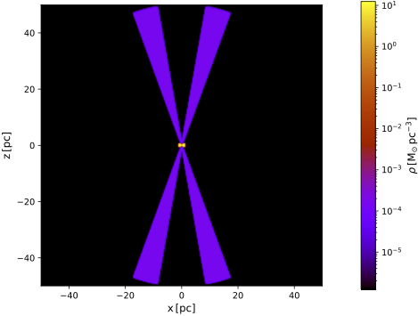
The figures below show a vertical cut and all-sky map using the density distribution gridded with an octree of 16 million cells (i.e. the simulation producing the polarization results shown in the above plot).
| Vertical cut through model using octree grid | Vertical cut zoomed in on central portion |
|---|---|
|
|
| All-sky optical depth at \(0.21~\mu\text{m}\) for model using octree grid |
|---|
|
It is evident that the cells of the octree, which are aligned with the Cartesian coordinate axes, are unable to properly resolve the slanted borders of the torus and cone geometry. Furthermore, the edges of the low-density cone are discretized with significantly larger cells than those of the torus. This is caused by the subdivision algorithm used by the SKIRT octree grid, which is mostly controlled by density and optical depth. Because the cone is 5 orders of magnitude less dense than the torus, it is exceedlingly hard to have the octree use smaller cells for the cone, unless by resolving the empty space in the model by a large number of unnecessarily small cells.
The polarization characteristics of the observed radiation in the models discussed here are dominated by scattering strengths and scattering angles, mostly off the low-density cone and perhaps the edges of the torus. This causes the results to be very sensitive to the precise geometry of the density distribution, and thus to its precise discretization. Because of the model's makeup, a grid defined in spherical coordinates is much better suited to do this well than a Cartesian octree. Note that this situation arises in part because the synthetic model specifies very steep (actually, infinite) gradients at the borders of the density distributions. Still, even in a more realistic setting, the Cartesian octree cells will have trouble "following" the slanted surfaces.
Congratulations, you made it to the end of this tutorial!