 |
The SKIRT project
advanced radiative transfer for astrophysics
|
|
The SKIRT project
advanced radiative transfer for astrophysics
|
In this tutorial you will explore options for extracting three-dimensional (3D) information from a simulated SKIRT model. You will use the output of a simple spiral galaxy simulation to produce volume- or mass-weighted temperature histograms and fully 3D temperature maps.
This tutorial assumes that you have completed the introductory SKIRT tutorials Monochromatic simulation of a dusty disk galaxy and Panchromatic simulation of a dust torus, and that you have reviewed the topics on Visualizing SKIRT results with PTS and Probes and forms, or that you have otherwise acquired the working knowledge introduced there. At the very least, before starting this tutorial, you should have installed the SKIRT code, and preferably also PTS and a FITS file viewer such as DS9 (see Installation Guide).
To avoid spending time creating yet another SKIRT parameter file from scratch, this tutorial offers a ski file for download to serve as an initial configuration. Download the file TutorialVolumetricSpiral.ski using the link provided in the table below and put it into your local working directory.
| Initial SKIRT parameter file | TutorialVolumetricSpiral.ski |
|---|
SKIRT simulations usually produce output through both instruments and probes. Instruments mimic the observation of radiation as projected on a plane. The output is therefore limited to two dimensions by definition. In contrast, probes can peek inside the simulated model and provide information on various physical quantities, such as the medium density or temperature. Because a probe has access to the full model, the output can take various forms, including arbitrary planar cuts or projections. Interestingly, a probe can also be configured to output information for each cell in the simulation's spatial grid, providing 3D data on the model. That is the topic of this tutorial.
There is an important caveat, however. The techniques discussed here only apply to quantities that are discretized on the internal spatial grid used for the radiative transfer simulations. Essentially, this includes all medium properties, whether derived (resampled) from the input model (e.g., density, velocity) or calculated in the simulation (e.g., radiation field, dust temperature). However, it does not include the properties of the primary sources (e.g., luminosity density), because these are never discretized on the internal spatial grid. Instead, the emitted photon packets are sampled directly from the original (possibly imported) definition of the primary sources.
Rename the downloaded SKIRT parameter file to a shorter name of your liking ending with the ".ski" filename extension, for example volume.ski. Open the ski file in a text editor and examine its contents. You should recognize the following configuration elements (not in this order):
ThemisDustMix with support for stochastically heated dust grains in the dust emission calculationRun the volume.ski ski file with SKIRT. If SKIRT immediately produces a fatal error while constructing the simulation, this probably means that the ski file needs upgrading; see Upgrading SKIRT parameter files.
Note the construction of the octree grid during setup. The total number of cells should be slightly over half a million; the precise number depends on random sampling effects. Because the simulation includes dust emission and we aim for a fairly well-resolved temperature distribution, the run time is a bit longer than usual for a tutorial.
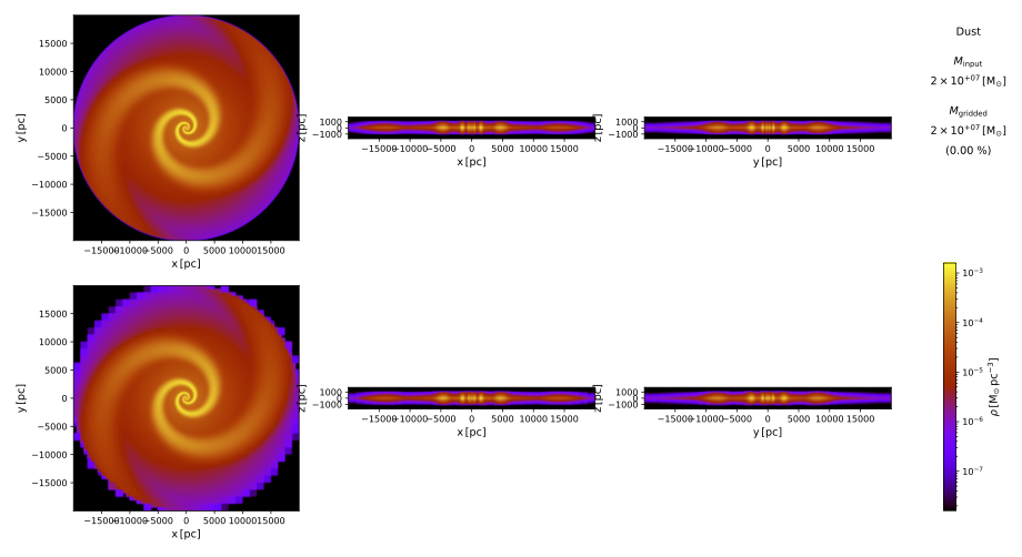
After the simulation completes, open the convergence info file volume_cnv_convergence.dat in a text editor and verify the statistics. The total dust mass should be accurately captured by the grid, with a discrepancy much smaller than 1 per cent. The optical depth along the coordinate axes may show discrepancies of up to about 5 per cent. These apparent inaccuracies are mostly a result of an implementation limitation in the spiral arm decorator: the redistribution of the dust mass from the disk into the stellar arms is not properly accounted for in the listed input optical depth.
Now use PTS to produce some standard plots and verify that the model behaves as expected. Because this is not the focus of this tutorial, the plots below are reproduced with limited resolution.
pts plot_convergence .
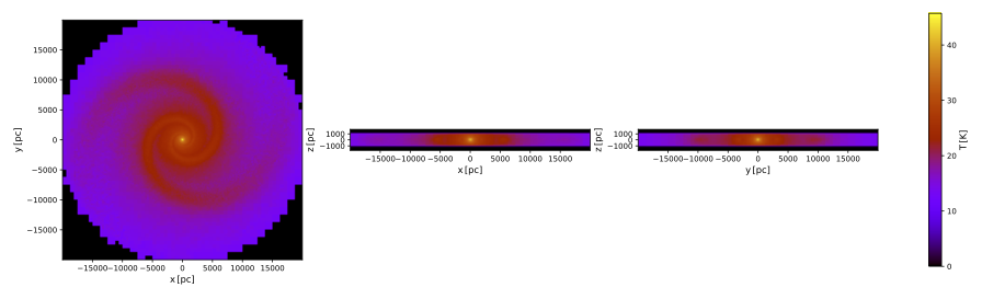
pts plot_temperature .
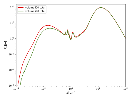
pts plot_seds .
It is instructive to inspect the header information in the column text files produced by the "per cell" probes:
$ head -5 volume_prp_cellprops.dat
# column 1: spatial cell index (1)
# column 2: x coordinate of cell center (pc)
# column 3: y coordinate of cell center (pc)
# column 4: z coordinate of cell center (pc)
# column 5: cell volume (pc3)
$ head -3 volume_tmp_dust_T.dat
# Indicative temperature per spatial cell
# column 1: spatial cell index (1)
# column 2: indicative temperature (K)
The "spatial cell properties" probe outputs columns with the coordinates of the cell center and the volume for each cell, plus some additional columns that are not of interest for this tutorial (but could be for other purposes). The temperature probe configured with the "per cell" form simply outputs the indicative dust temperature for each cell. Combining the information in both files allows obtaining 3D volumetric information.
The first column in each file lists an index that identifies the spatial cell represented by this row. In the current implementation of the probes, there is always a row for each cell and the rows are representing the cells in the same order. As a result, there is no need for explicit synchronization through the cell index.
You can now use Python to load and analyze these data. The code snippets shown below depend on at least some of the previous snippets and thus should be entered sequentially. To work through the tutorial, you can copy each new code section into a regular Python script and run the partially complete program from the start. Alternatively, you can copy the code sections into a Python notebook so that you can run each section separately.
At the start, import the Python packages used for handling the data and for plotting.
Read the relevant columns into numpy arrays. Verify that all arrays have the same length, equal to the total number of spatial cells listed in the log file.
To get a feel for the data, generate some basic histograms.
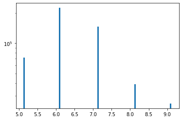
This plot shows that the cell volume distribution has a limited number of discrete values, and that those values differ by a factor of \(2^3\). This is as expected for an octree grid, where nodes are recursively subdivided into 8 subnodes until some termination criterion has been reached.
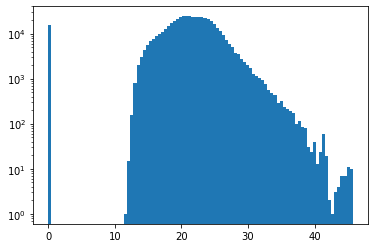
The indicative dust temperature values calculated by the simulation range from 11 to 45 K. Keep in mind that this plot shows the temperature distribution of the spatial cells, regardless of their size. It thus heavily depends on the discretization used in the simulation. See below for a histogram with a more appropriate physical interpretation.
There is also a significant number of cells with zero temperature. It turns out that these cells do no contain any dust; this can be verified by removing the cells with zero density from the histogram (not shown here).
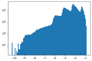
To allow showing the density on a logarithmic axis, this code removes empty cells before plotting the histogram. The density values have a wide dynamic range of 7 orders of magnitude. Again, this plot shows the density distribution of the spatial cells, regardless of their size and thus heavily depends on the discretization used in the simulation.
Now you can produce histograms with a more appropriate physical interpretation by combining information from the various probes.
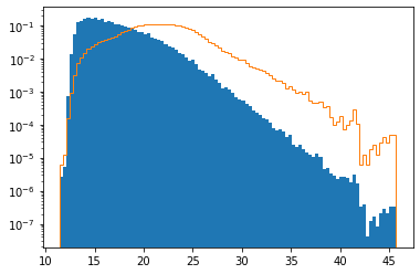
This plot shows the volume-weighted temperature distribution (solid blue) versus the purely cell-based temperature distribution considered in the previous paragraph (orange curve). Both distributions are normalized for ease of comparison. Compared to the physically meaningful volume-weighted distribution, the cell-based distribution is significantly shifted to higher temperatures. This indicates that higher-temperature regions are discretized with smaller and thus more numerous cells.
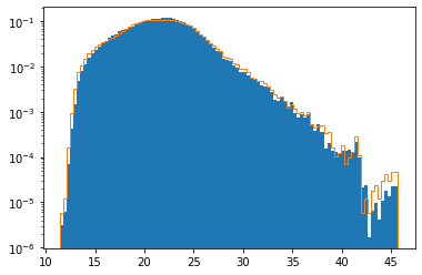
This plot shows the mass-weighted temperature distribution (solid blue) versus the purely cell-based temperature distribution (orange curve), again both normalized. The two distributions are surprisingly similar. This can be understood by realizing that the octree subdivision criteria are designed to place a roughly equal amount of mass in each cell.
Using only a slightly more involved Python script, you can generate a simple 3D map of the indicative dust temperature calculated by SKIRT for the model.
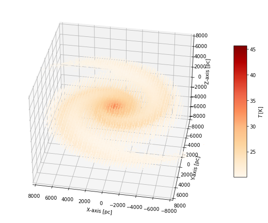
The low-temperature cut-off of 20 K causes the cells on the outskirts of the galaxy model to be omitted from the plot, providing a clearer focus on the inside regions. You may want to study the effect of adjusting some of the hard-coded values, including the temperature cutoff, the 3D inclination and azimuth, and the size of the axis box.
As shown here, the plot does not take into account the cell sizes. This can be mitigated by varying the size of the markers (determined by the s argument) with the cell volume. However, for this example the effect is small because the plot is mostly showing inner cells with comparable volumes. Also, in this plot, the high-temperature markers in the center of the model are in part obscured by the surrounding lower-temperature markers. This can be mitigated by employing a color map that includes transparency for the colors representing lower temperatures. These embellishments are outside the scope of this tutorial.
The marker positions in the 3D plot above are determined by the cell centers in the spatial grid of the simulation. For a typical SKIRT simulation grid, this means the markers are unevenly spread over the domain because there are more (smaller) cells in high-density regions. In some cases, it may be preferable to instead place markers at set of predefined positions, for example the points on a regular grid. Similary, other applications may require obtaining the value of physical quantities at a set of predefined positions of interest.
One option is to configure a probe with the AtPositionsForm probe form and provide a text column file listing the coordinates of the query points. In this case, SKIRT will perform the sampling and produce an output file with the required values.
Another option is to query the 3D data discussed in this tutorial. In an octree grid, each cell has the same form factor as the complete spatial domain. Given the cell centers and volumes, one can thus reconstruct the cell bounding boxes, which allows determining the cell containing a given query location. For a limited number of queries, a brute force algorithm looping over all cells might be acceptable. For a larger number of queries, a more sophisticated search mechanism would be required.
While this would be feasible, you can achieve approximate results through a much simpler approach. The Python scipy package implements efficient nearest neighbor querying using a tree-based mechanism. You can employ this mechanism to quickly find the cell center nearest to the query point. For an octree grid, this does not always correspond to the cell containing the query point: at the interface between cells of a different subdivision level, the nearest cell center may be the center of a neighboring cell. However, this approximation may be acceptable in many applications.
For example, the following Python code retrieves the indicative dust temperature at the origin of the model coordinate system from the 3D data loaded earlier in this tutorial.
Which should print a number in the high temperature range, e.g.:
45.57380517
To finalize this tutorial, it is instructive to perform the same simulation and data analysis using a different type of spatial grid. Specifically, replacing the hierarchical octree grid with an unstructured Voronoi grid offers some valuable insights.
To this end, copy the ski file you have been using to another name and/or directory, and in the new file replace the 5 lines defining the octree grid and its subdivision policy by the following definition of a Voronoi grid:
<VoronoiMeshSpatialGrid minX="-2e4 pc" maxX="2e4 pc" minY="-2e4 pc" maxY="2e4 pc" minZ="-1750 pc" maxZ="1750 pc"
    policy="DustDensity" numSites="500000" filename="" relaxSites="true"/>
This specifies a Voronoi grid with a half a million cells (roughly the number of cells in the octree) constructed from sites that are randomly sampled from the dust density distribution in the model. In other words, there will be more, smaller cells in high-density regions.
Now run SKIRT with the new, adjusted ski file. Once the simulation completes, perform the same data analysis as presented in the previous sections of this tutorial. The results should be similar to those of the octree simulation. However, you should find some differences as indicated below.
Congratulations, you made it to the end of this tutorial!