 |
The SKIRT project
advanced radiative transfer for astrophysics
|
|
The SKIRT project
advanced radiative transfer for astrophysics
|
This topic provides an overview of SKIRT's capabilities for importing sources and media from snapshots produced by hydrodynamical simulations. The discussion is organized as follows:
Computer programs that simulate the time-evolution of astrophysical systems produce increasingly realistic numerical models. The scale of the models varies substantially between these simulations (e.g., stellar system, star forming region, galaxy, cosmological box), as does the set of included physics (e.g., dark and baryonic matter, gravity, hydrodynamics, magnetic fields, star formation and stellar feedback, chemical evolution, radiative energy transfer, dust formation and destruction). Regardless, we refer to these programs as hydrodynamical simulation codes.
Hydrodynamical simulations usually output a series of snapshots, describing the state of the simulated model at a particular time in its evolution, including the spatial distribution and other relevant properties of the dynamical components, such as for example the stars and the interstellar medium in a galaxy.
Because of the nonlocal and nonlinear behavior of radiation transport, predicting the observable properties of these hydrodynamical models requires a full, three-dimensional radiative transfer simulation in all but the most trivial cases. Assuming that the radiation crossing times are much shorter than the dynamical time scales, the radiative transfer simulation can be performed as a post-processing step based solely on the information contained in a particular snapshot. The post-processing procedure extracts the spatial distribution of the radiation sources and the obscuring medium, plus the corresponding properties, from the hydrodynamical snapshot data, and then performs a radiative transfer simulation on the resulting setup.
Hydrodynamical simulation codes historically employ one of two schemes: a Lagrangian formulation based on moving particles (smoothed particle hydrodynamics or SPH) or a Eulerian approach based on a non-moving spatial grid, often an adaptive grid with multiple refinement levels (AMR). Some more recent codes introduce a new scheme that employs a moving mesh based on a Voronoi tessellation of the spatial domain. This new scheme is claimed to combine the best features of SPH and the traditional Eulerian approach, and it is becoming increasingly popular. Other codes use a meshless approach based on a set of discretization locations reminiscent of Voronoi generator sites.
Most codes represent the collisionless components (dark matter, stars) as particles handled by an N-body solver, even if the hydrodynamical solver for the collisional components (gas, dust) is mesh-based.
The relevant snapshot data must be provided for import into SKIRT using one of the supported column text file formats. In other words, an external procedure (usually a Python script) is needed to extract the appropriate information from the native snapshot data and output the result as a column text file. While this seems restrictive, it is almost never an issue in practice. In most cases, one needs to perform some additional processing anyway, such as locating the proper data files, performing a coordinate transformation, limiting the imported data to a given aperture, calculating indirectly derived properties, etc. Furthermore, the alternative would be to implement a variety of data formats and point SKIRT to the relevant data through a potentially very complex configuration mechanism that would never be as flexible as the Python language.
In all cases, the columns in the text file must be in the order prescribed by the SKIRT component controlling import of the file (see Importing media and Importing sources below). The values in each column can be provided either in the default units prescribed by that SKIRT component, or in the units defined through header lines in the data file being imported (see the TextInFile class). In the latter case, any of the supported units corresponding to the imported quantity can be used (see The SKIRT units system & supported units).
The heart of the SKIRT snapshot import mechanism is implemented by the classes in the following hierarchy.
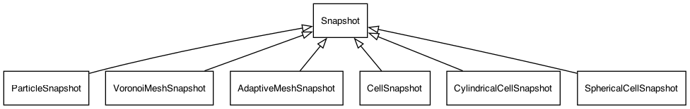
The Snapshot subclasses support several paradigms for describing the spatial geometry of an imported source or medium component:
It is perfectly possible to mix and match these options in the same simulation. For example, it is quite common to import radiation sources using particles and medium densities using a mesh-based grid.
The Snapshot classes are not exposed to the user through the SKIRT parameter file. Instead, they are invoked under the hood by the various components that are user-configured. Three distinct, parallel class hierarchies make use of the Snapshot classes, as summarized in the table below.
Each of these class hierarchies implements the appropriate layer of functionality on top of the Snapshot classes. For example, sources can launch photo packets, media can quickly find the material density at a given location, and geometries offer a density distribution normalized to unity. The latter can be used for importing either source or medium components and may be useful in some specific cases.
Any nontrivial SKIRT simulation includes one or more medium components describing the transfer medium in the model (see the Medium class and its subclasses). Each medium component defines (a) the spatial density distribution of the medium and (b) the relevant material properties of the medium at each location.
We first examine the most common situation where a medium component is assigned material properties that do not vary across the spatial domain (although different medium components may be assigned different material properties). In this case, SKIRT offers three distinct ways to define a component's medium density distribution:
In any case, each medium component must be assigned a specific material mixture, i.e. one of the subclasses of the MaterialMix class, which defines the optical and calorimetric properties of the medium, considered to be constant across the spatial domain.
On the other hand, for some simulations it is desired to associate spatially variable material properties with a medium component. For example, the snapshot may define a specific dust grain material or a different dust grain size distribution for each cell or particle. This advanced feature is supported only when configuring one of the ImportedMedium subclasses (i.e. the first option in the list above). For more information and examples, refer to Spatially varying the dust mix in imported models, which is the second part of the tutorial Configuring custom dust mixes.
We first consider the case of an SPH simulation that does not separately track the dust component. We thus need a heuristic to derive the dust density from the gas density. Several possible prescriptions have been described in the literature, and these are most easily implemented in the (Python) procedure that prepares the snapshot data for SKIRT import. However, for compatibility with previous versions, SKIRT optionally supports a basic scheme that assumes the amount of dust to be proportional to the metal fraction in the gas, except in areas where the gas is too hot to form dust. Here is an example column text file that defines two gas particles and includes the particle properties required to implement this scheme:
# example1.txt: import file for particle media -- dust
# Column 1: position x (pc)
# Column 2: position y (pc)
# Column 3: position z (pc)
# Column 4: smoothing length (pc)
# Column 5: gas mass (Msun)
# Column 6: metallicity (1)
# Column 7: temperature (K)
# Column 8: velocity vx (km/s)
# Column 9: velocity vy (km/s)
# Column 10: velocity vz (km/s)
0 0 0 1  10  0.02   35  0 0 10
0 0 9 2   5  0.01 9000  0 0 -9
This file could be imported using the following configuration in the parameter file:
<ParticleMedium filename="example1.txt" massType="Mass" massFraction="0.3"
                importMetallicity="true" importTemperature="true" maxTemperature="500 K" importVelocity="true"
                importMagneticField="false" importVariableMixParams="false" useColumns="">
    <smoothingKernel type="SmoothingKernel">
        <CubicSplineSmoothingKernel/>
    </smoothingKernel>
    <materialMix type="MaterialMix">
        <MeanInterstellarDustMix/>
    </materialMix>
</ParticleMedium>
The first five columns in the file specify the particle position, smoothing length and mass. These columns must always be present. The subsequent columns specify the metallicity, the temperature, and the components of the bulk velocity. The presence of these columns depends on the values of the respective importXXX options in the parameter file.
In case both metallicity and temperature are imported, as in the example, the dust mass corresponding to each particle is calculated as
\[ M_\mathrm{dust} = \begin{cases} f_\mathrm{mass}\,Z\,M_\mathrm{gas} & \mathrm{if}\; T<T_\mathrm{max} \\ 0 & \mathrm{otherwise} \end{cases} \]
where \(M_\mathrm{gas}\), \(Z\), and \(T\) are the gas mass, metallicity, and temperature given by the particle's properties in the import file, and \(f_\mathrm{mass}\) and \(T_\mathrm{max}\) are constant values specified in the parameter file. Hence, we obtain 0.06 solar masses for the first particle, and zero for the second particle because its temperature is above the cutoff value. If the metallicity is not imported, its value is taken to be unity in the formula above; if the temperature is not imported or if the maximum temperature is set to zero, there is no temperature cutoff. If neither metallicity or temperature are imported, and the mass fraction is set to one, the dust mass equals the mass specified in the import file. Note that, for dust media, the imported metallicity and temperature values are never retained in the simulation; they are discarded after being used to determine the dust mass.
The total medium density at an arbitrary position is then obtained through
\[ \rho(\mathbf{r}) = \sum_{j=1}^N M_j \, W(|\mathbf{r}-\mathbf{r}_j|,h_j) \]
where \(M_j\) indicates the dust mass of each particle and \(W(r,h)\) is the radial density profile of the smoothing kernel.
The ParticleMedium class allows configuring one of several spherically symmetric smoothing kernels, including the frequently-used cubic spline kernel (the CubicSplineSmoothingKernel class) and a scaled Gaussian smoothing kernel (the ScaledGaussianSmoothingKernel class). Corresponding to the kernels used in SPH simulations, these kernels have a finite support so that only a relatively small number of terms in the sum above have a non-zero contribution. SKIRT uses this property to accelerate the calculation of the medium density at a given spatial position even for a potentially large number of smoothed particles.
If the bulk velocity components are imported, the simulation will take into account the Doppler shift caused by the velocity of the medium relative to the model coordinate system when interacting with photon packets.
For more information on the importMagneticField option, see Emission from aligned spheroidal dust grains. For more information on the importVariableMixParams option, see Spatially varying the dust mix in imported models. For more information on the useColumns option, see the TextInFile::useColumns() function.
Electrons and gas media can be imported using the ParticleMedium class in a similar manner, but there are a few differences. Most importantly, if provided, metallicity and/or temperature are no longer used to adjust the mass value and they are instead imported as regular properties of the medium. That is, these quantities are stored in the medium state of each spatial cell and can thus be used during the simulation, for example to help determine a cross section or to emulate thermal motion. Here is an example column text file that defines two particles representing electrons:
# example2.txt: import file for particle media -- electrons
# Column 1: position x (pc)
# Column 2: position y (pc)
# Column 3: position z (pc)
# Column 4: smoothing length (pc)
# Column 5: nr of electrons (1)
# Column 6: temperature (K)
# Column 7: velocity vx (km/s)
# Column 8: velocity vy (km/s)
# Column 9: velocity vz (km/s)
0 0 0 1  1e30  3e6  0 0 10
0 0 9 2  5e31  7e5  0 0 -9
This file could be imported as follows:
<ParticleMedium filename="example2.txt" massType="Number" massFraction="1"
                importMetallicity="false" importTemperature="true" maxTemperature="0 K" importVelocity="true"
                importMagneticField="false" importVariableMixParams="false" useColumns="">
    <smoothingKernel type="SmoothingKernel">
        <CubicSplineSmoothingKernel/>
    </smoothingKernel>
    <materialMix type="MaterialMix">
        <ElectronMix includePolarization="false" includeThermalDispersion="true" defaultTemperature="1e4 K"/>
    </materialMix>
</ParticleMedium>
Because the massType option has been set to Number, the electron mass corresponding to each particle is calculated as
\[ M_\mathrm{e} = f_\mathrm{mass} N_\mathrm{e} m_\mathrm{e} \]
where \(f_\mathrm{mass}\) is specified in the parameter file, \(N_\mathrm{e}\) is the number of electrons taken from the import file, and \(m_\mathrm{e}\) is the electron rest mass. The mass fraction \(f_\mathrm{mass}\) is usually set to unity, but could be used to specify some fraction if desired. The imported temperature is retained for use during the simulation to emulate the appropriate thermal motion of the electron population in each spatial cell.
In general, the rules for electrons and gas media are as follows; for details see the material mix class being used.
Mass or Number. For the latter, the mass is obtained by multiplying the imported number by the mass of the species handled by the material mix (electron, hydrogen atom, ...).Some hydrodynamical simulation codes use Voronoi tessellations for spatial discretization. Although the mesh may move as the simulated model evolves over time, each snapshot is defined on a particular, well-defined mesh.
A Voronoi tessellation partitions the spatial domain in convex polyhedra. Consider a given set of points in the domain, called sites. For each site there will be a corresponding region consisting of all points in the domain closer to that site than to any other. These regions are called Voronoi cells, and together they form the Voronoi tessellation of the domain. Due to the nature of a Voronoi tessellation, the geometry of the grid is completely defined by the positions of the generating sites. It is hence not necessary for a snapshot to store, for example, vertices and edges of the cells.
Similar to the approach for other snapshot types, the VoronoiMeshMedium class expects a column text file with a line for each cell. The first three columns list the coordinates of the generating site for the cell, and the subsequent columns specify the relevant physical cell properties. Compared to Particle media – dust and Particle media – electrons and gas, this corresponds to omitting the particle smoothing length. The Voronoi cells are reconstructed from the positions of the generating sites, and the density and other properties are assumed to be uniform across the polyhedral volume of each cell.
The VoronoiMeshMedium places the generating sites in a cuboidal spatial domain; the domain walls serve as the external boundary for the Voronoi cells in the outer layers. This bounding box must be specified in the parameter file. For example, here is an import file that defines the dust mass density in seven Voronoi cells:
# example5.txt: import file for Voronoi mesh media -- dust
# Column 1: position x (pc)
# Column 2: position y (pc)
# Column 3: position z (pc)
# Column 4: dust mass density (Msun/pc3)
 0.255   0.352   0.774   0.112
-0.557   0.826  -0.933   0.635
-0.664  -0.644  -0.493   0.952
-0.848   0.909   0.015   0.757
 0.441  -0.801  -0.743   0.822
 0.784   0.476   0.458   0.975
-0.154  -0.408   0.863   0.034
In this example, the dust medium has no bulk velocity and the procedure writing the import file included the actual dust mass density after deriving it from the snapshot data using an appropriate heuristic. The file could be imported using:
<VoronoiMeshMedium filename="example5.txt"
                   minX="-1 pc" maxX="1 pc" minY="-1 pc" maxY="1 pc" minZ="-1 pc" maxZ="1 pc"
                   massType="MassDensity" massFraction="1"
                   importMetallicity="false" importTemperature="false" maxTemperature="0 K" importVelocity="false"
                   importMagneticField="false" importVariableMixParams="false" useColumns="">
    <materialMix type="MaterialMix">
        <MeanInterstellarDustMix/>
    </materialMix>
</VoronoiMeshMedium>
Again, the massType can be specified as MassDensity, NumberDensity, Mass or Number as for Cell media and Adaptive mesh media. The other medium properties, including metallicity, temperature, and velocity, can be specified as described in Particle media – dust and Particle media – electrons and gas.
Because the VoronoiMeshSnapshot class builds the structure of the mesh during import, it is possible to use the imported Voronoi grid during the simulation's radiative transfer phase; see Configuring the spatial grid.
This section discusses an issue that leads to unexpected results when importing subvolumes extracted from a larger Voronoi grid.
Consider a hydrodynamical simulation that employs a Voronoi tessellation for discretizing the medium density distribution. The procedure for extracting a gravitationally bound structure (such as a galaxy) from a snapshot may produce a set of cells covering an irregularly shaped volume. When importing this structure, SKIRT will recreate the cells on the outskirts of the volume so that they fill the simulation's spatial domain – which, by definition, is always a cuboid. This is inevitable because SKIRT sees only the Voronoi sites inside the imported volume.
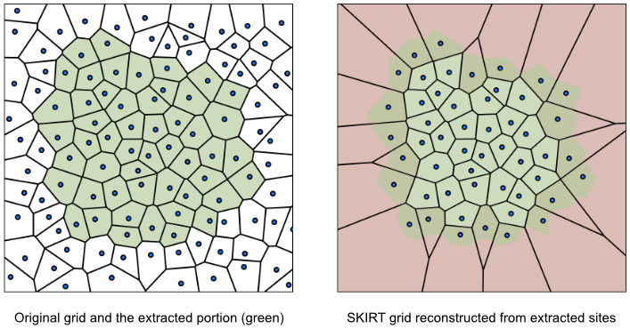
The process is illustrated with a 2D example in the diagram above. The left panel represents the (complete or partial) simulation volume defined in the snapshot. The colored cells represent the gravitationally bound structure extracted from the snaphot. The import file presented to SKIRT thus contains the Voronoi sites corresponding to the colored cells, but not the sites corresponding to the uncolored cells. Assuming the SKIRT spatial grid fully encloses the imported structure, SKIRT is forced to create new Voronoi cells at the outer edges. The right panel shows the SKIRT grid with green color covering the shape as it was in the snapshot and red color covering the enlarged cells.
Now assume that each cell (site) in the import file specifies an associated medium density, and that the ski file accordingly specifies the massType as MassDensity. Because the reconstructed cells in the outskirts are so much larger, with uniform density, they will contain an excessive amount of mass that no longer corresponds to the definition in the snapshot. This will in turn lead to incorrect simulation results.
The following actions should be taken to mitigate this problem:
Mass (and adjust the data in the import file accordingly). This causes total mass to be preserved, although some of the mass in the outskirts will be smeared out over the larger reconstructed cells.Simulations with an adaptive mesh paradigm use a hierarchical grid that is refined to a variable level depending on the resolution requirements in various regions of the model. While the resolution requirements and thus the grid may change as the system evolves, each particular snapshot corresponds to a unique and well-defined hierarchical grid. Thus, an adaptive mesh snapshot includes some description of the structure of the hierarchical grid, implicitly or explicitly defining the spatial extent of each grid cell, and for each cell the values of a suite of physical properties.
While it is possible to use this technique with spherical or cylindrical coordinate systems, perhaps to benefit from certain quasi-symmetries in the model, SKIRT only supports adaptive mesh snapshots using Cartesian coordinates (but see Cell media for an alternative solution). In a Cartesian hierarchical grid, the cuboidal spatial domain is recursively subdivided into smaller cuboids according to some scheme until the desired resolution in each region is reached.
The AdaptiveMeshMedium class expects a text file in a format that describes the topological structure of the Cartesian hierarchical grid and lists the relevant physical properties in each cell, as described in the AdaptiveMeshSnapshot class documentation. In short, the hierarchical grid structure is organized into a tree with nonleaf and leaf nodes. These nodes can be arranged in a linear sequence using so-called Morton ordering. The complete topology is defined by the information in the non-leaf nodes (lines starting with an exclamation point in the SKIRT text format) in combination with the Morton ordering. The leaf nodes require no further geometric information and are thus represented by regular column text rows listing just the physical quantities to be imported. For example, here is a trivial import file that defines two cells representing electrons:
# example4.txt: import file for adaptive mesh media -- electrons
# Column 1: nr of electrons (1)
# Column 2: temperature (K)
# Column 3: velocity vx (km/s)
# Column 4: velocity vy (km/s)
# Column 5: velocity vz (km/s)
! 2 1 1
1e30  3e6  0 0 10
5e31  7e5  0 0 -9
Because the import file does not contain any coordinates, the size of the spatial domain must be defined separately in the SKIRT configuration file. The above example file could be imported as follows:
<AdaptiveMeshMedium filename="example4.txt"
                    minX="-1 pc" maxX="1 pc" minY="-0.5 pc" maxY="0.5 pc" minZ="-0.5 pc" maxZ="0.5 pc"
                    massType="Number" massFraction="1"
                    importMetallicity="false" importTemperature="true" maxTemperature="0 K" importVelocity="true"
                    importMagneticField="false" importVariableMixParams="false" useColumns="">
    <materialMix type="MaterialMix">
        <ElectronMix includePolarization="false" includeThermalDispersion="true" defaultTemperature="1e4 K"/>
    </materialMix>
</ParticleMedium>
The massType can be specified as MassDensity, NumberDensity, Mass or Number as described for Cell media. The other medium properties, including metallicity, temperature, and velocity, can be specified as described in Particle media – dust and Particle media – electrons and gas.
Because the AdaptiveMeshSnapshot class preserves the topological structure during import, it is possible to use the imported AMR grid during the simulation's radiative transfer phase; see Configuring the spatial grid. On the other hand, providing the cells in Morton order might be a complicated task, depending on the structure of the original snapshot data. In that case, the CellMedium class discussed in the next section offers an excellent alternative.
Many hydrodynamical simulation codes use spatial cells with boundaries that are lined up with the coordinate axes. With Cartesian coordinates, all cells then are cuboids or "boxes". With cylindrical coordinates, cells are bounded by cylinders and planes, and with spherical coordinates, cells are bounded by spheres, cones and planes. The CellMedium, CylindricalCellMedium, and SphericalCellMedium classes can import media defined on such grids regardless of the topological structure of the grid, because each cell is handled as a seperate entity. The approach is similar to what has been described for particles in the previous sections (Particle media – dust and Particle media – electrons and gas) with the following important differences:
MassDensity or NumberDensity in addition to Mass or Number, because the cell volume is defined unambiguously.For example, here is column text file that defines two cuboidal cells containing dust:
# example3.txt: import file for cell media -- dust
# column 1: xmin (pc)
# column 2: ymin (pc)
# column 3: zmin (pc)
# column 4: xmax (pc)
# column 5: ymax (pc)
# column 6: zmax (pc)
# Column 7: gas mass (Msun/pc3)
# Column 8: metallicity (1)
# Column 9: temperature (K)
# Column 10: velocity vx (km/s)
# Column 11: velocity vy (km/s)
# Column 12: velocity vz (km/s)
-1 -0.5 -0.5  0 0.5 0.5   0.1  0.02   35  0 0 10
 0 -0.5 -0.5  1 0.5 0.5   0.5  0.01 9000  0 0 -9
This could be imported using:
<CellMedium filename="example3.txt" massType="MassDensity" massFraction="0.3"
            importMetallicity="true" importTemperature="true" maxTemperature="500 K" importVelocity="true"
            importMagneticField="false" importVariableMixParams="false" useColumns="">
    <materialMix type="MaterialMix">
        <MeanInterstellarDustMix/>
    </materialMix>
</CellMedium>
As noted in the Media overview, as an alternative to using one of the ImportedMedium subclasses, the configuration can instead include a GeometricMedium with the corresponding ImportedGeometry subclass.
The expected text file then has a format similar to that described above for the ImportedMedium subclasses, but without support for the bulk velocity or any of the other additional medium properties. Furthermore, the ImportedGeometry subclasses always normalize the total mass of the density distribution to unity, as required for all geometries. This means that the actual total mass must be provided through one of the standard normalization mechanisms offered by the GeometricMedium class.
It is usually more convenient to use the ImportedMedium subclasses, except in cases where the mass normalization is not known when the import file is being written.
Every SKIRT simulation that includes media requires a spatial grid for use during the simulation's radiative transfer phase. This grid should be properly configured to provide adequate spatial resolution in areas with high medium densities or steep density gradients, and at the same time avoid placing cells in less important regions.
When importing a hydrodynamical simulation snapshot, often the best option is to select an adaptive grid, such as an octree grid (PolicyTreeSpatialGrid) or a Voronoi grid (VoronoiMeshSpatialGrid). To help evaluate and configure the quality of a spatial grid, it is instructive to review the convergence information and the density cuts along the coordinate planes generated by SKIRT upon request. For more information and examples, see the tutorial Building a proper spatial grid for a spiral galaxy.
For mesh-based hydrodynamical snapshots as described in Voronoi mesh media and Adaptive mesh media, SKIRT offers the option to directly adopt the imported grid for performing radiative transfer rather than constructing a new one. This avoids resampling the medium density and other properties, which may introduce inaccuracies and takes time. In other words, it ensures that the radiative transfer simulation uses the exact same snapshot representation as the hydrodynamical simulation. On the other hand, it is not always the best choice. The resolution requirements for the radiative transfer treatment may differ from those for the hydrodynamical simulation. The optimal overall resolution might differ, and fine-grained cells may be needed in different areas of the domain. Also, sometimes the spatial domain used for radiative transfer can be made smaller than the full snapshot domain, cutting off the outer regions that do not contain significant amounts of material anyway. And finally, the PolicyTreeSpatialGrid class (offering octree or binary tree grids) is highly optimized for tracing photon packets, so the photon shooting simulation phase might be substantially faster.
For cell-based hydrodynamical snapshots as described in Cell media, SKIRT does not receive any information on the original structure of the grid, i.e. the hierarchical or neighboring relationships between the cells. It is not possible to use such a set of unrelated cells as a grid for tracing photon packets. Instead, the imported model must be regridded to one of SKIRT's regular spatial grids, just as when importing particles. When importing a model in Cartesian coordinates, the hierarchical octree or binary tree grids offered by the PolicyTreeSpatialGrid class are often the best choice. When importing a model in cylindrical or spherical coordinates, it might be beneficial to configure a Cylinder3DSpatialGrid or Sphere3DSpatialGrid with mesh points that match (some of) the cell borders of the imported discretization.
During a SKIRT simulation, all physical quantities are assumed to be uniform across each cell of the spatial grid used for radiative transfer. After constructing that spatial grid, SKIRT establishes the average medium properties in each cell by sampling the values from the input model, i.e. the medium components configured for the simulation.
The SamplingOptions class offers a number of configuration options related to this sampling process. A separate number of spatial samples per grid cell can be configured for the density and for all of the the other medium properties (as a group). In each case, if the specified number of samples is one, the property is sampled just at the central position of the cell. If the specified number is larger than one, the property is sampled at the given number of positions, randomly selected from a uniform distribution within the cell volume, and the average value of these random samples is used.
There is just a single bulk velocity value per spatial cell. If multiple medium components specify a bulk velocity, the values sampled from these components are aggregated using one of three possible policies: Average, Maximum, or First.
Any nontrivial SKIRT simulation includes one or more components describing the radiation sources in the model (see the Source class and its subclasses). Each source component defines (a) the spatial density distribution of the sources and (b) the spectral energy distribution (SED) at each location. SKIRT offers three distinct ways of accomplishing this:
These options can be mixed at will with multiple source components. For example, one could augment the stellar sources imported from a spiral galaxy snapshot with a built-in point source representing an active galactic nucleus.
As noted in the introduction (Hydrodynamical simulations), most hydrodynamical simulation codes represent source components such as stellar populations as particles, even if the hydrodynamics is mesh-based.
A particle snapshot consists of a set of smoothed particles, each characterized by a list of properties. Formally, the spatial luminosity distribution (at a particular wavelength) in a particle snapshot is defined by a list of \(N\) particles and an assumed smoothing kernel \(W(r,h)\), with each smoothed particle characterized by a position \(\mathbf{r}_j\), a smoothing length \(h_j\), and a luminosity contribution \(L_j\). The total luminosity density at an arbitrary position \(\mathbf{r}\) is then given by
\[ \Sigma(\mathbf{r}) = \sum_{j=1}^N L_j \, W(|\mathbf{r}-\mathbf{r}_j|,h_j) \]
The ParticleSource class allows configuring one of several spherically symmetric smoothing kernels, including the frequently-used cubic spline kernel (the CubicSplineSmoothingKernel class) and a scaled Gaussian smoothing kernel (the ScaledGaussianSmoothingKernel class).
The ParticleSource class expects a column text file with a single line for each particle. The first four columns specify the central position and the smoothing length of the particle. The number and interpretation of the subsequent columns depends on the SED family configured for this ParticleSource instance. For example, for the Bruzual-Charlot SED family (BruzualCharlotSEDFamily), the remaining three columns provide the properties of the stellar population represented by the particle, including the initial mass of the stellar population (at the time it was born) and the metallicity and current age of the stellar population. For information on the parameters required for other SEDFamily subclasses, refer to the corresponding class documentation.
The ParticleSource class can also be configured to take into account the Doppler shift caused by the velocity of the radiation sources relative to the model coordinate system. If this option is enabled, the input text file must provide three additional columns (after the smoothing length and before the additional properties for the SED family), specifying the vector components of the particle's bulk velocity, and optionally a fourth column specifying the velocity dispersion of sources within the extent of the particle.
The default units for these quantities can be overridden by including columns header info in the file as described in the TextInFile class header. For example, here is an import file describing just a single source particle placed at the origin of the model coordinate system, moving in the direction of the vertical axis:
# example6.txt: import file for particle source
# Column 1: position x (pc)
# Column 2: position y (pc)
# Column 3: position z (pc)
# Column 4: smoothing length (pc)
# Column 5: velocity vx (km/s)
# Column 6: velocity vy (km/s)
# Column 7: velocity vz (km/s)
# Column 8: mass (Msun)
# Column 9: metallicity (1)
# Column 10: age (Gyr)
0 0 0 1  0 0 50  10  0.01  5
This file could be imported as follows:
<ParticleSource filename="example6.txt" importVelocity="true" importVelocityDispersion="false"
                importCurrentMass="false" useColumns="" sourceWeight="1" wavelengthBias="0.5">
    <smoothingKernel type="SmoothingKernel">
        <CubicSplineSmoothingKernel/>
    </smoothingKernel>
    <sedFamily type="SEDFamily">
        <BruzualCharlotSEDFamily imf="Chabrier" resolution="Low"/>
    </sedFamily>
</ParticleSource>
Even if the stellar populations (or other radiation sources) in a hydrodynamical simulation are represented as "smoothed particles" with a finite extent defined by some spherical kernel, these collisonless particles do not conform to the semantics of the collisional particles employed in smoothed particle hydrodynamics (SPH). Indeed, the smoothing length for SPH particles is determined so that neighboring particles overlap sufficiently to achieve a smooth combined density field. For the collisonless stellar particles, there is no such requirement. As a result, the simulation often does not track (and thus does not output) a particle property that directly corresponds to a smoothing length that can be used for import into SKIRT. In other words, an appropriate smoothing length must be "fabricated". There is, unfortunately, no single best way to do this.
In a SKIRT simulation, the smoothing length for stellar particles is not intended to achieve an overly smooth luminosity field. If the smoothing lengths are an order of magnitude larger than the typical distance between particles or the typical medium cell size, there is a risk of losing the geometrical effects of the star/dust interplay. In fact, as long as the smoothing lengths are sufficiently small, their precise values do not seem to significantly affect the integrated SED of the simulated model. However, they do affect the realism of the generated synthetic images.
Let us consider the options. First, note that many N-body solvers in hydrodynamical simulations use gravitational softening to avoid extreme close encounters between the particles, which would cause numerical instabilities. The corresponding softening length is sometimes stored in the snaphot data, but it is usually not appropriate as a substitute for smoothing length in the context of SKIRT import.
The easiest option is to specify a fixed smoothing length for all particles. This works as long as the value is not too large, but it produces somewhat artificial-looking images. This can be improved by introducing some randomness. One could simply sample the value from some distribution, but that feels very arbitrary. Or one could determine the value as a function of, for example, the current mass of the particle (as opposed to the initial mass which must be passed to the stellar population SED templates).
Some hydrodynamical simulations keep track of a stellar particle "smoothing length" that determines the sphere of influence for stellar feedback. The volume within this radius would include a given number of eligible neighboring gas particles or cells (as opposed to stellar particles). One could use this smoothing length, or a fixed fraction thereof, for import into SKIRT. Unfortunately, the value tends to grow very large in under-resolved areas, such as on the outskirts of a galaxy, producing artificially large stellar blobs in the images. Putting a cap on the value could counter this.
Another option is to calculate a smoothing length after the fact by including a given number of neighboring stellar particles in the corresponding volume. This calculation is not trivial but quite feasible with the appropriate Python packages. It also suffers from the same problem in under-resolved areas as described above unless counter-measures are taken.
Lastly, one could resample a subset or all of the particles similar to what has been described in the literature, e.g. by Camps et al. 2016. In short, the procedure splits the young stellar particles, which are few in number but still dominant in the shorter wavelengths, into smaller particles with molecular cloud-like masses. These sub-particles are then spread out in time and space and assigned smoothing lengths based on their masses.
It is best to experiment with these or other options and evaluate what works to satisfaction depending on the needs of the study at hand.
Although used less frequently, SKIRT fully supports importing sources that are represented on a grid through the VoronoiMeshSource, AdaptiveMeshSource, CellSource, CylindricalCellSource, and SphericalCellSource classes. The import file format is a blend of what has been described in previous sections:
For more information, refer to those sections and to the documentation of the various imvolved classes.
If the hydrodynamical simulation does not track the relevant properties for defining the local emission spectrum, one can still import the spatial luminosity distribution from the snapshot and assign a built-in SED that is constant across the spatial domain. This is achieved by combining the GeometricSource class with one of the ImportedGeometry subclasses. This option does not allow importing velocity information, although it is still possible to assign a global, built-in velocity vector field to the imported source.
In the import text file, the SED family parameters are replaced by a single column specifying the luminosity contribution of the particle. This value can be given in arbitrary units because the ImportedGeometry classes normalize the total luminosity to unity as is required for all geometries. Because of this normalization, the actual luminosity of the source must be configured through one of the regular normalization options offered by the GeometricSource class.
Note that the ImportedGeometry subclasses offer some options for compatibility with medium density distributions (see Geometric media) that are irrelevant in the context of source luminosities and thus should be disabled. For mesh-based imported geometries, the massType option behaves as follows:
Mass and Number, the value in the import file indicates the relative luminosity contribution of the cell;MassDensity and NumberDensity, the value in the import file is multiplied by the volume of the cell to determine the cell's relative luminosity contribution.