In this tutorial you are faced with a snapshot exported from a 2D hydrodynamical model. The model is defined in the meridional plane using cylindrical coordinates. The snapshot provides both density and velocity distributions. Assuming a central point source, the goal is to investigate the effect of the kinematics on the observed spectrum at various inclinations.

Along the way, you will:

prepare raw data for import into SKIRT,
configure a SKIRT simulation for importing 2D cylindrical data,
configure a cylindrical radiative-transfer grid appropriate for the imported data,
provide support for kinematics (i.e. bulk velocities),
plot and interpret some of the simulation results.

Getting ready

This tutorial assumes that you have completed the introductory SKIRT tutorials Monochromatic simulation of a dusty disk galaxy and Panchromatic simulation of a dust torus, and that you have reviewed the topics on Importing snapshots, Adjusting column order in import files, and Spatial grids and meshes overview, or that you have otherwise acquired the working knowledge introduced there. At the very least, before starting this tutorial, you should have installed the SKIRT code, and preferably also PTS and a FITS file viewer such as DS9 (see Installation Guide).

Begin by downloading the ski file and the raw data file used in this tutorial using the first two links provided in the table below. If you want (or need) to skip the data preparation step, you can also download the import-ready data file using the third link provided in the table below.

Ski file	TutorialCylindrical.ski
Raw data	TutorialCylindricalRawData.txt
Import-ready data	TutorialCylindricalImportReady.txt

Prepare the raw data for import

The raw data file comes with the following description.

""The data represents the density and velocity of the material in an axi-symmetric wind solution near an AGN. There is an opening funnel region near the symmetry axis, which could be predominantly occupied by jets (not part of this model). The file contains the following 6 columns, in this order:

cylindrical radius $R / R_{in}$
cylindrical axial distance $z / R_{in}$
wind density $\log (n / n_{in})$
$v_{R} / c$
$v_{φ} / c$
$v_{z} / c$

Herein $R_{in} = 9 \times 10^{13} cm$ , $n_{in} = 10^{12} {cm}^{- 3}$ , and $c$ is the speed of light. The wind velocity components are “capped” at $0.99 c$ in this non-relativistic framework. The spatial grid is given by $Δ (\log R) = 0.1$ and $Δ (\log z) = 0.1$ .""

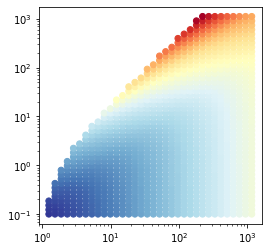
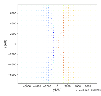
To get some insight in the data, make a quick and dirty plot using a simple python script, for example:

import numpy as np
import matplotlib.pyplot as plt
import matplotlib
 
cmap = matplotlib.cm.get_cmap('RdYlBu')
normalizer = matplotlib.colors.Normalize()
 
R,z,n,_,_,_ = np.loadtxt("TutorialCylindricalRawData.txt", unpack=True)
 
plt.xscale('log')
plt.yscale('log')
plt.scatter(R,z, color=cmap(normalizer(n)))
plt.show()

This yields:

The SKIRT class CylindricalCellMedium imports a density distribution defined in cylindrical coordinates. However, it requires a list of cylindrical cells lined up with the cylindrical coordinate axes rather than a set of data points. You thus need to convert each of the data points in the raw data file to a cylindrical cell that encloses the point. This can be accomplished with a fairly straightforward python script as follows:

import numpy as np
 
# load raw data
R, z, n, vR, vphi, vz = np.loadtxt("TutorialCylindricalRawData.txt", unpack=True)
 
# R borders
logR = np.log(R)
logRgrid = np.unique(logR)
logRshift = (logRgrid[1]-logRgrid[0])/2
Rmin = np.exp(logR - logRshift)
Rmax = np.exp(logR + logRshift)
 
# z borders
logz = np.log(z)
logzgrid = np.unique(logz)
logzshift = (logzgrid[1]-logzgrid[0])/2
zmin = np.exp(logz - logzshift)
zmax = np.exp(logz + logzshift)
 
# scale to SKIRT units
R_in = 9e13 # cm
n_in = 1e12 # cm^-3
c = 2.99792458e8 # m/s
 
Rmin *= R_in
Rmax *= R_in
zmin *= R_in
zmax *= R_in
n = np.exp(n) * n_in
vR *= c
vphi *= c
vz *= c
 
# write header info
outfile = open("TutorialCylindricalImportReady.txt", 'wt')
outfile.write("# SKIRT-ready data for cylindrical import tutorial\n")
outfile.write("# Column: box Rmin (cm)\n")
outfile.write("# Column: box zmin (cm)\n")
outfile.write("# Column: box Rmax (cm)\n")
outfile.write("# Column: box zmax (cm)\n")
outfile.write("# Column: number density (1/cm3)\n")
outfile.write("# Column: velocity R (m/s)\n")
outfile.write("# Column: velocity phi (m/s)\n")
outfile.write("# Column: velocity z (m/s)\n")
 
# write positive and negative z-axis
np.savetxt(outfile, np.array((Rmin, zmin, Rmax, zmax, n, vR, vphi, vz)).T, fmt="%20.14e")
np.savetxt(outfile, np.array((Rmin, -zmax, Rmax, -zmin, n, vR, vphi, -vz)).T, fmt="%20.14e")
outfile.close()
 
# print information to help configuring the spatial grid in SKIRT
print ("R: {:1.12e} .. {:1.12e} cm".format(Rmin.min(), Rmax.max()))
print ("   use LogMesh with {:1d} bins and central bin fraction {:1.12e}".format(1+len(logRgrid), Rmin.min()/Rmax.max()))
print ("z: {:1.12e} .. {:1.12e} cm (mirrored)".format(zmin.min(), zmax.max()))
print ("   use SymLogMesh with {:1d} bins and central bin fraction {:1.12e}".format(1+2*len(logzgrid), zmin.min()/zmax.max()))

After loading the raw data, the script builds a cylindrical cell around each grid point by shifting the cell borders by half of the bin width in logarithmic space. It then scales the data values to SKIRT-supported units, using the normalization constants given in the description accompanying the raw data file. Finally the script outputs the result as a text file including header information for each column in SKIRT format. In fact, each cell is written twice, mirroring the material distribution about the equatorial plane. At the very end, the script prints some information to the console that will help configuring the spatial grid in SKIRT, as will be discussed later in this tutorial:

R: 1.008235702265e+14 .. 1.157281232035e+17 cm
   use LogMesh with 34 bins and central bin fraction 8.712106222376e-04
z: 8.114174078163e+12 .. 1.119638154725e+17 cm (mirrored)
   use SymLogMesh with 93 bins and central bin fraction 7.247139661970e-05

Configure the SKIRT simulation

The ski file for this tutorial is offered for download through the link at the start of this page. Although this avoids spending time on entering all the required details, it is important to understand the various elements of the configuration as discussed below. As is often the case for complex configurations, this ski file was constructed in several phases. First, we used the console Q&A (or MakeUp) to generate the basic structure with the appropriate source and medium components, and with just a few instruments and probes. We then manually edited the ski file to improve readability, removing some default elements and wrapping long lines. Finally we filled in the appropriate numbers for things that are hard to get right in one go (domain sizes, field of views, grid details) and we added the desired instruments and probes by copying and adjusting those already there. When introducing a new type of instrument or probe, we consulted the ski file reference in the online documentation to find the precise class and property names. Alternatively, we sometimes used the console Q&A or MakeUp to construct a dummy ski file that contained the desired elements and manually copied them over into the target ski file.

Open the downloaded ski file in a text editor and follow along with the discussion below.

Front matter

<MonteCarloSimulation userLevel="Regular" simulationMode="ExtinctionOnly" numPackets="1e7">
    <units type="Units">
        <StellarUnits wavelengthOutputStyle="Wavelength" fluxOutputStyle="Frequency"/>
    </units>

We want to simulate the effects of the medium extinction and kinematics on the radiation emitted by a central point source. There is no need for secondary emission, so the simulation mode is set to extinction-only. The number of photon packets can be adjusted to achieve a desired level of Monte Carlo noise in the results. We selected stellar units because of the size of the object under consideration. The flux output style is a matter of preference.

Source

<PointSource positionX="0 pc" positionY="0 pc" positionZ="0 pc"
             velocityX="0 km/s" velocityY="0 km/s" velocityZ="0 km/s"
             sourceWeight="1" wavelengthBias="0">
    <sed type="SED">
        <SingleWavelengthSED wavelength="0.55 micron"/>
    </sed>
    <normalization type="LuminosityNormalization">
        <LineLuminosityNormalization wavelength="0.55 micron" luminosity="1 Lsun"/>
    </normalization>
</PointSource>

The point source is stationary at the model origin. For an actual science case, we would configure a spectrum that is relevant for the object under study. For this tutorial, however, the point source emits at a single optical wavelength, making it easy to study the effects of the moving medium in the observed spectra. Note that SingleWavelengthSED is a subclass of LineSED, corresponding to a luminosity normalization using LineLuminosityNormalization. The actual normalization value is arbitrary since all observed fluxes scale linearly with the source luminosity.

Medium

<CylindricalCellMedium filename="TutorialCylindricalImportReady.txt"
        autoRevolve="true" numAutoRevolveBins="32" massType="NumberDensity" massFraction="3e-7"
        importMetallicity="false" importTemperature="false" maxTemperature="0 K"
        importVelocity="true" importMagneticField="false" importVariableMixParams="false"
        useColumns="*0">
    <materialMix type="MaterialMix">
        <MeanInterstellarDustMix/>
    </materialMix>
</CylindricalCellMedium>

We use a CylindricalCellMedium to import the 2D density and velocity distribution defined in the prepared import file. The autoRevolve flag is enabled to automatically revolve the meridional plane around the vertical axis. While the density is axially symmetric and thus constant with azimuth, the velocity vectors are rotated and thus do change with azimuth. Consequently, it is important for the grid to properly resolve the velocity field in the azimuthal direction. The value of the numAutoRevolveBins property controls this discretization. The number 32 seems reasonable but remains arbitrary.

Because the snapshot data being imported represents gas around an AGN, it provides number densities as hydrogen atoms per unit of volume. For this tutorial we instead insert a basic dust model. We further specify an arbitrary, very small mass fraction to bring the optical depth of the system down to a reasonable value (see the optical depth map produced by SKIRT, shown later in this tutorial). While this is obviously artificial, it limits the simulation run time and simplifies the interpretation of the results.

The importVelocity is enabled to properly handle the velocity columns. All other flags are disabled.

Very importantly, the useColumns property is set to a value of "*0". This causes the import procedure to automatically look for matching column names in the import file header and allows the missing azimuth columns to be automatically replaced by zeroes, as required by the CylindricalCellMedium for 2D import. When using "*0", always verify the column assignments listed in the simulation log file during setup:

Column 1: box Rmin <-- box Rmin (cm)
Column 2: box phimin <-- 0
Column 3: box zmin <-- column 2: box zmin (cm)
Column 4: box Rmax <-- column 3: box Rmax (cm)
Column 5: box phimax <-- 0
Column 6: box zmax <-- column 4: box zmax (cm)
Column 7: number density <-- column 5: number density (1/cm3)
Column 8: velocity R <-- column 6: velocity R (m/s)
Column 9: velocity phi <-- column 7: velocity phi (m/s)
Column 10: velocity z <-- column 8: velocity z (m/s)

Spatial Grid

<Cylinder3DSpatialGrid minRadius="0 cm" maxRadius="1.157281232035e+17 cm"
                       minZ="-1.119638154725e+17 cm" maxZ="1.119638154725e+17 cm">
    <meshRadial type="Mesh">
        <LogMesh numBins="35" centralBinFraction="8.712106222376e-04"/>
    </meshRadial>
    <meshAzimuthal type="Mesh">
        <LinMesh numBins="32"/>
    </meshAzimuthal>
    <meshZ type="Mesh">
        <SymLogMesh numBins="93" centralBinFraction="7.247139661970e-05"/>
    </meshZ>
</Cylinder3DSpatialGrid>

The CylindricalCellMedium class treats the cylindrical cells in the import file as separate, individual entities. This means that cells can be listed in arbitrary order, cells covering empty regions of the domain can be omitted, and cells can even overlap (although that is not recommended). While SKIRT can import information in this manner, such a set of unrelated cells is not suitable for tracing photon packets while performing radiative transfer. SKIRT thus always uses a distinct internal spatial grid optimized to perform radiative transfer, and thus requires regridding the imported distribution on this internal grid.

It would be perfectly possible to use one of the regular or hierarchical Cartesian grids offered by SKIRT, or perhaps a Voronoi grid. However, regridding the imported distribution (defined on a cylindrical grid) would introduce additional inaccuracies and noise to the simulation model. We instead aim to perfectly match the imported grid by configuring a Cylinder3DSpatialGrid with the appropriate properties. This is possible because SKIRT offers many flexible ways to position the cell borders in each coordinate direction through one of the Mesh subclasses. In this case, the python script used to prepare the import data file also calculated the domain borders, number of bins, and central bin fraction for the logarithmic grid in the radial and vertical directions. We merely need to copy the values. The aximuthal grid simply matches the 32 bins specified for the auto-revolve feature of the CylindricalCellMedium class.

Instruments

<FrameInstrument instrumentName="xy" distance="10 pc" inclination=" 0 deg" azimuth="  0 deg" roll="90 deg"
        fieldOfViewX="2.32e17 cm" numPixelsX="500" centerX="0" fieldOfViewY="2.32e17 cm" numPixelsY="500" centerY="0"
        recordComponents="true" numScatteringLevels="0" recordPolarization="false" recordStatistics="false">
    <wavelengthGrid type="WavelengthGrid">
        <PredefinedBandWavelengthGrid includeGALEX="true" includeSDSS="true" include2MASS="true"/>
    </wavelengthGrid>
</FrameInstrument>

We configured a FrameInstrument parallel to each Cartesian coordinate plane with a field of view that covers the full model and using 10 standard broadbands in the UV to NIR range, in hopes of capturing the kinematic structure of the model. The recordComponents flag is enabled because the scattered component avoids the direct radiation from the central source, which can be annoying in the total flux for sight-lines with low or no extinction.

<SEDInstrument instrumentName="i05" distance="10 pc" inclination="05 deg" azimuth="0 deg" roll="0 deg" radius="0 pc"
        recordComponents="false" numScatteringLevels="0" recordPolarization="false" recordStatistics="false">
    <wavelengthGrid type="WavelengthGrid">
        <LogWavelengthGrid minWavelength="0.03 micron" maxWavelength="3 micron" numWavelengths="300"/>
    </wavelengthGrid>
</SEDInstrument>

We further included an SEDInstrument for each of four inclinations. The wavelength range was adjusted to include the red- and blueshifted fluxes observed from the model, based on early simulation runs.

Probes

<ImportedMediumDensityProbe probeName="imp_dns_cut">
<ImportedMediumVelocityProbe probeName="imp_vel_cut">
<DensityProbe probeName="grd_dns_cut" aggregation="Type" probeAfter="Setup">
<VelocityProbe probeName="grd_vel_cut">
<OpacityProbe probeName="grd_opa_pro" wavelength="0.55 micron" aggregation="Type" probeAfter="Setup">

We configured various probes to help evaluate our model setup (shown partially above; please refer to the ski file). Most importantly, we included density and velocity cuts on both the imported and internal grid. This allow us to verify whether we succeeded in exactly matching these grids. The opacity probe uses an all sky projection to show optical depth viewed from the center of the model. The results of these probes are shown in the following sections.

Interpret the simulation results

Run the simulation. It is often handy to place the output files in a separate directory:

$ skirt -o out TutorialCylindrical

With $10^{7}$ photon packets, the simulation runs for about 2 minutes on a recent powerful desktop computer.

Density

First have a look at the output of the ConvergenceInfoProbe. The input and gridded mass should be equal because we exactly matched both grids. The optical depth along each of the coordinate axes is zero because the distribution is discretized on a logarithmic grid, which leaves a thin empty slice in its center.

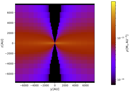
Now plot the density cuts using the following PTS command, and/or have a look at the FITS files produced by the ImportedMediumDensityProbe and the DensityProbe:

$ pts plot_density out --dex 2

Both density cuts look exactly the same because we did properly match the internal grid to the import grid. The distribution also nicely follows the plot of the raw data points you made earlier in this tutorial. One of the vertical cuts is shown below.

Optical depth

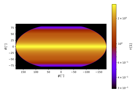
Have a look at the FITS file produced by the OpacityProbe probe paired with the AllSkyProjectionForm, or plot the optical depth using:

$ pts plot_opacity out --dex 1

As shown below, the result is obviously axi-symmetric. The radial optical depth reaches a maximum of about 3 near the equitorial plane.

Velocity

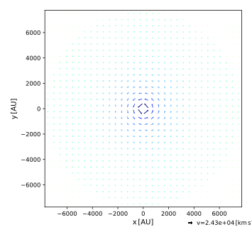
Plot the cuts through the velocity field using:

$ pts plot_velocity out --bin 64

Again, the imported and gridded results match perfectly, as expected. Two of the cuts are shown below.

Obervables

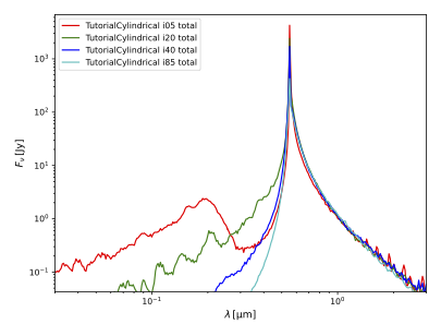
Plot the spectra generated by the SEDInstrument instances:

$ pts plot_sed out --wmin 0.03 --wmax 3

As shown below, the blueshift significantly depends on inclination, while the redshift does not.

Open the primaryscattered FITS files for the various FrameInstrument instances and scroll through the wavelength bands to get an impression of the kinematical structure of the medium.

Congratulations, you made it to the end of this tutorial!